Unsupervised Learning: Clustering
Our discussion of how training data can be used to categorize customer comments based on sentiment (positive, negative, and neutral).
Airline contexts include punctuality, food, comfort, entertainment, etc. An owner can determine which areas of his business need to be focused on by using this analysis. His priority would be the quality of food being served to customers if, for example, the most negative comments are about food. There are situations, however, in which business owners are uncertain. It is also possible to lack training data. In addition, frames of reference can change. Unknown target classes can’t be classified using algorithms. These situations require clustering algorithms. Wine-making uses clustering where clusters represent brands of wine, and wines are grouped according to their component ratio. A classification algorithm can recognize a type of image, but an algorithm has to separate images with multiple shapes that have the same image. This type of use case uses clustering algorithms.
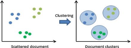
Based on similarity or distance measures, clustering groups objects. This is an unsupervised learning example. Clustering differs from classification in that target classes are well-defined. A target class’ characteristics are determined by its training data and models. Therefore, classification is supervised. Alternatively, clustering uses similarity and distance to define meaningful classes. This figure shows how documents are clustered.
Clustering using K-Means
Consider a retail distributor with an online system where local agents manually enter trading information. It requires them to fill out a field called City. Due to the fact that the data entry process is manual, people normally make a lot of spelling mistakes. As an example, people enter Dehi instead of Delhi, Dehli instead of Delly, and so on. Due to the fact that the number of clusters is already known, the retailer can attempt to solve this problem using clustering. A K-means clustering example.
Two inputs are required for the K-means algorithm. A set of N vectors is called data X, and a set of clusters is called K, which represents how many clusters need to be created. As a result, each vector in X has a label indicating the points assigned to each cluster as well as a set of K centroids in each cluster. Unlike any other centroid, the centroid of a cluster is closest to its points. The condition for the K clusters Ck and the K centroids μ k can be expressed as follows: minimize
with respect to C k , μ k .
Polynomial time cannot be used to solve this optimization problem. As a solution, Lloyd suggests an iterative process. In this method, two steps are iterated until the solution is reached.
There are K centroids, and each point is assigned to a particular cluster or centroid, whose distance from the point concerned is the minimum.
Using the following formula, it recalculates the centroid of each cluster:
Until no further rearranging of cluster points is necessary, the two-step procedure continues. There is no guarantee that the algorithm will converge, but a local minimum may be reached.
For performing K-means clustering in Python, here is a simple implementation of Lloyd’s algorithm:
There is, however, one limitation to K-means clustering. Consider a scenario in which all of your data points are located in eastern India. To begin the K=4 clustering process, you choose a randomly selected center from Delhi, Mumbai, Chennai, and Kolkata. Because all your points are in eastern India, they are always assigned to Kolkata since it is the closest. This results in a one-step convergence of the program. It is run multiple times and averaged to avoid this problem. Centroids can be initialized in the first step using various tricks.
The Elbow Method for Choosing K
K-means clustering requires you to determine K in certain cases. A percentage of variance is used as a variable depending on the number of clusters in the elbow method. A number of clusters are initially selected. A second cluster is added, which does not make the data modeling much better. At this point, the elbow criterion is used to determine the number of clusters. The “elbow” cannot always be identified unambiguously. In percentages, variance is calculated as the ratio of the between-group variance of individual clusters to the total variance. Take the previous example, where the retailer operates in four cities: Delhi, Kolkata, Mumbai, and Chennai. Since the programmer is unaware of that, he plots the variance percentage by clustering with K=2 to K=9. In this case, K=4 is clearly the right number for K based on the elbow curve he gets.
Measure of similarity or distance
Clustering relies on a measure of distance or similarity. In this section, I will explain how distance and similarity are measured. Here’s what distance actually means.
Characteristics
Following are the properties of distances:
There can only be a dist(x, y) of 0 if and only if x = y.
dist(x, y) > 0 when x ≠ y.
dist(x, y) = dist(x, y).
dist(x,y) + dist(y,z) >= d(z,x) for all x, y, and z.
Euclidean distance and general distance
It is the length of the geometrical line between p and q that determines the distance between them. (
. This is called Euclidean distance.
When p = (p1, p2,…, p n) and q = (q1, q2,…, q n) are Euclidean n-space points, the Pythagorean theorem provides the distance (d) between these two points:
In Euclidean n-space, a Euclidean vector represents the position of a point. Measures are based on the magnitude of vectors. The following formula is used to calculate its length:
There is a direction and a distance associated with a vector. As shown here, the distance between two points, p and q, may have a direction, and so another vector can be used to represent it:
q — p = (q1–p1, q2–p2, …. , q n –p n )In Euclidean distance terms, the distance (or displacement) vector from point p to point q is the Euclidean length.
The dimensions are as follows:
The two dimensions are as follows:
Assuming that p = (p1, p2) and q = (q1, q2) in the Euclidean plane, then the distance is as follows:
d(p,q) = √(q1–p1)² + (q2–p2)²From the equation, the distance between two points is the product of the polar coordinates of p and q.
√r1² + r2² — 2r1r2cos(θ1 − θ2)In n dimensions:
Distances are generally calculated as follows:
D2(p,q) = (p1 — q1)2 + (p2 — q2)2 + … + (p i — q i )2 + … + (p n — q n )2.Distance squared according to Euclidean geometry
It is possible to square the standard Euclidean distance in order to place progressively greater weight on objects that are further apart. As a result, we have the following equation:
d2(p,q) = (p1 — q1)2 + (p2 — q2)2 + … + (p i — q i )2 + … + (p n — q n )2.Due to the triangle inequality, squared Euclidean distance cannot be considered a metric. On the other hand, it is often used in optimization problems in which only distances are to be compared.
The distance between string edits
Dissimilarity between two strings is measured by edit distance. To make two strings identical, it counts the minimum number of operations required. A misspelled word may be identified by automatic spelling corrections by using edit distance. The edit distance can be divided into two types.
Levenshtein edit distance
Needleman edit distance
Levenshtein Distance
When two words are changed into each other, the Levenshtein distance is the least number of insertions, deletions, or replacements needed. Vladimir Levenshtein was the first to consider this distance in 1965.
In addition to Levenshtein distance, edit distance might refer to a larger family of distance metrics. Alignment of pair-wise strings is associated with it.
Using the following five edits as an example, the Levenshtein distance between Calcutta and Kolkata is 5:
Calcutta → Kalcutta (substitution of C for K)Kalcutta → Kolcutta (substitution of a for o)Kolcutta → Kolkutta (substitution of c for k)Kolkutta → Kolkatta (substitution of u for a)Kolkatta → Kolkata (deletion of t )There are several simple upper bounds to the Levenshtein distance when the strings are identical, and the lower bounds are zero when the strings are not identical. A code example for Levinstein distance is given in the code for K-mean clustering.
The Needleman-Wunsch algorithm
The Needleman–Wunsch algorithm aligns nucleotide or protein sequences in bioinformatics. Dynamic programming was used for the first time to compare biological sequences. The program is dynamically programmed. In the first step, a matrix is created with alphabets as rows and columns. There is a similarity score associated with each alphabet in each row and column of the matrix. A score is either matched, not matched, or matched with an insert or deletion. A backtracing operation is done from the bottom-right to the top-left cell of the matrix and a path is found that has the lowest neighbor score distance. Needleman-Wunsch distance is calculated by adding up the scores of the backtracing paths.
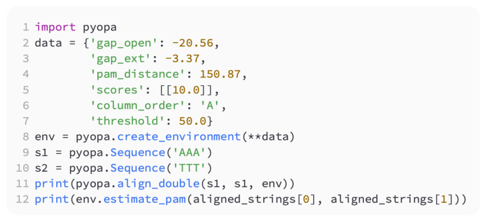
Needleman-Wunsch distances between strings are provided by Pyopa, a Python module.
In spite of the simplicity of Levenshtein’s implementation and lower computational cost, Needleman-Wunsch’s algorithm is more efficient when you want to introduce a gap in string matching (for example, Delhi and Delhi).
Documents with similar contexts
The similarity between two documents indicates how similar they are. A similarity score of 1 indicates maximal similarity, with a similarity range of [-1,1] or [0,1].
Similarities
Documents are analyzed as vectors of terms excluding stop words in order to measure similarity. Let’s say A and B represent two documents. Using a similarity metric in this case, we can see the following:
Dice
The Dice coefficient is denoted by the following:
sim(q,dj) = D(A,B) =
Also,
and let
Overlap
The Overlap coefficient is computed as follows:
Sim(q,dj) = O(A,B) =
The Overlap coefficient is calculated using the max operator instead of min.
Jaccard
The Jaccard coefficient is given by the following:
Sim(q,dj) = J(A,B) =
The Jaccard measure signifies the degree of relevance.
Cosine
The cosine of the angle between two vectors is given by the following:
Sim(q,dj) = C(A,B) =
There is a difference between distance and similarity. A similarity measure would be numeric data correlation, while a distance measure would be Euclidian distance. Distance has no upper boundary, whereas the similarity measure has a range between 0 and 1. The degree of similarity may be negative, but the degree of distance cannot be negative by definition. Researchers are continuously finding new distance measures for various applications despite almost the same clustering algorithms as at the beginning of the field.
How Does Hierarchical Clustering Work?
The process of hierarchical clustering involves iteratively clustering data objects. In general, there are two types.
A bottom-up approach or a hierarchical aggregation algorithm
Top-down algorithms, or dividing hierarchies


