

Unsupervised Machine Learning Algorithms
Unsupervised machine learning algorithms are discussed in this article. Unsupervised learning techniques are introduced at the beginning of the article.

Our next topic is clustering: k-means and hierarchical clustering. In the next section, we examine a dimensionality reduction algorithm, which can be helpful when we have a large number of input variables. Using unsupervised learning for anomaly detection is illustrated in the following section. Association rules mining is one of the most powerful unsupervised learning techniques. Furthermore, this section explains how associations discovered through association rules mining can help us make data-driven decisions by providing interesting relationships between the various data elements across transactions.
Writing this indepth article takes time and research. If you can help then please consider becoming a member for just $5 a month using this this link. It really helps me a lot and keeps me going and you will get most in depth article everyday + interview questionarie (coming very soon) everyday directly to your email inbox. It is our goal to provide the reader with a clear understanding of how unsupervised learning can be applied to a variety of real-world problems by the end of this article. The reader will gain an understanding of the basic algorithms and methodologies used in unsupervised learning today.
This article covers the following topics:
Unsupervised learning
Clustering algorithms
Dimensionality reduction
Anomaly detection algorithm
Association rules mining
Introducing unsupervised learning
Unsupervised learning is the process of discovering and utilizing inherent patterns in unstructured data in order to provide some form of structure to the data. In the multidimensional problem space, if data were not produced by a random process, some patterns would appear between its data elements. A dataset is structured by using patterns discovered by unsupervised learning algorithms. A diagram illustrating this concept can be found below:
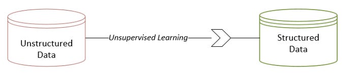
As a result of unsupervised learning, new features are discovered from existing patterns, which adds structure.
Data mining and unsupervised learning
An overview of the overall data-mining life cycle is essential to understanding unsupervised learning. Data mining can be divided into different phases through different methodologies. The data-mining life cycle can be represented in two ways at present:
The life cycle of CRISP-DM (Cross-Industry Standard Process for Data Mining)
An approach to data mining known as SEMMA (Sample, Explore, Modify, Model, Access)
In the early 1990s, Chrysler and SPSS (Statistical Package for Social Science) formed a consortium to develop CRISP-DM. Statistical Analysis System (SAS) proposed SEMMA. In order to understand the place of unsupervised learning in the data-mining life cycle, let’s look at one of these two representations, CRISP-DM. Within its life cycle, SEMMA has some similar phases.
This figure illustrates the six phases of the CRISP-DM life cycle:
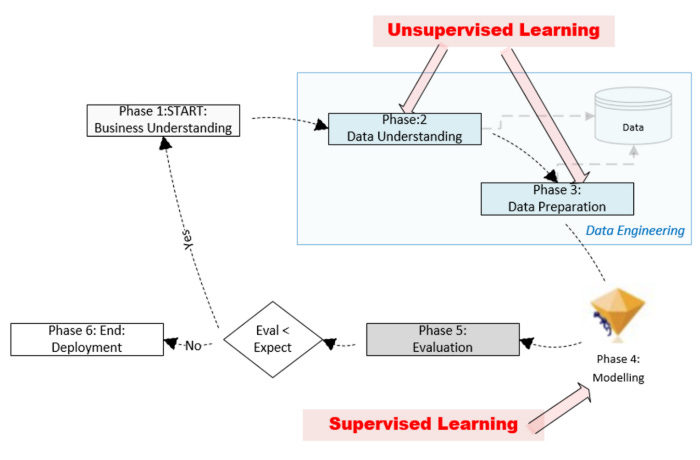
The phases are as follows:
First Phase: Gathering Business Requirements: This involves fully understanding the problem from a business perspective. It is important to define the problem scope and rephrase it in accordance with machine learning (ML) — for example, in the case of binary classification, it may be helpful to rephrase the requirements in terms of a hypothesis that can be proven or rejected. As part of this phase, we also document our expectations for the machine learning model that will be trained downstream in Phase 4 — for instance, we document the minimum accuracy of the model that can be deployed in production for a classification problem.
CRISP-DM’s Phase 1 is about understanding the business. The focus of the document is on what needs to be done, not how it will be accomplished.
The second phase is to understand the data that can be mined for data. Our goal in this phase is to determine if the right datasets are available for solving the problem. Having identified the datasets, we need to understand their quality and structure. Data analysis can provide us with important insights if we discover patterns that can be extracted out of it.
Additionally, we will try to identify a feature that can be used as a label (or target variable) based on Phase 1 requirements. Phase 2 objectives can be achieved using unsupervised learning algorithms. The following purposes can be achieved with unsupervised algorithms:
Analyzing the dataset to find patterns
Analyzing the discovered patterns allows us to understand the dataset’s structure
Identifying or determining the target variable
This phase prepares the data for the ML model we will train in Phase 4. There are two unequal parts to the available labeled data. Phase 4 involves training the model downstream with the larger portion of training data. A smaller portion of the data is used for model evaluation in Phase 5. This step involves preparing the data for training using unsupervised machine learning algorithms — for example, by converting unstructured data into structured data, providing additional dimensions.
The fourth phase involves modeling the discovered patterns through supervised learning. The data must be prepared in accordance with the requirements of the supervised learning algorithm we have chosen. It is also during this phase that the specific feature that will serve as the label will be identified. Phase 3 consisted of testing and training sets. During this phase, we formulate mathematical formulas for representing our patterns of interest. Phase 3 created the training data that was used to train the model. We will need to choose an algorithm that will result in a corresponding mathematical formulation.
In phase 5, test data from Phase 3 are used to evaluate the newly trained model. The evaluation must be repeated if it meets the expectations set in Phase 1, starting with Phase 1. An illustration of this can be seen in the image below.
A trained model is deployed in production once it meets or exceeds the expectations described in Phase 5, so it can begin generating solutions to the problem defined in Phase 1.
It is the task of Phase 2 (Data Understanding) and Phase 3 (Data Preparation) of the CRISP-DM life cycle to understand the data and prepare it for training. During these phases, data is processed. This data engineering phase is sometimes handled by specialists in an organization.
Solutions to problems are clearly driven by data. A workable solution is formulated using supervised and unsupervised machine learning. In this article, we examine the unsupervised learning component of the solution.
A significant portion of the machine learning process is the data engineering phase, which includes Phase 2 as well as Phase 3. A typical ML project can require up to 70% of the time and resources. A significant role can be played by unsupervised learning algorithms in data engineering.
Details regarding unsupervised algorithms can be found in the following sections.
Examples of practical applications
In marketing segmentation, fraud detection, and market basket analysis, unsupervised learning is commonly used to provide data with more structure. Here are some examples.
Voice categorization
A voice file can be classified using unsupervised learning. Using the fact that each person’s voice is unique, it creates potentially separable audio patterns. This technique is used by Google Home devices to distinguish between different people’s voices based on these patterns. Each user’s response will be personalized once Google Home has been trained.
For example, imagine we have a recorded conversation of three people chatting for half an hour. This dataset can be analyzed using unsupervised learning algorithms to identify the voices of distinct people. We are adding structure to unstructured data through unsupervised learning. We can rely on this structure to gain insights and prepare data for our chosen machine learning algorithm by adding additional dimensions to our problem space. Voice recognition is based on unsupervised learning as shown in the diagram below:
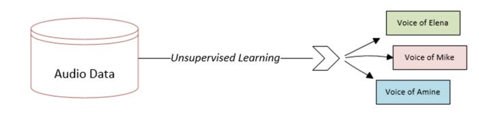
The unsupervised learning in this case suggests that we add a three-level feature.
Categorization of documents
A dataset of unstructured textual data can also be used for unsupervised machine learning, for example if the dataset consists of PDF documents, unsupervised learning can be used for:
Explore the dataset to discover a variety of topics
Each PDF document should be associated with a topic that was discovered
As shown in the following figure, unsupervised learning can be used to classify documents. Here is another example of how we are structuring unstructured data:
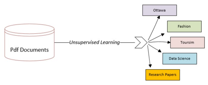
Document classification using unsupervised learning (Figure 6.4)
According to unsupervised learning, we should add a new feature with five distinct levels in this case.
Algorithms for clustering
An unsupervised learning technique based on clustering algorithms is one of the simplest and most powerful. Using it, we can understand what is happening in the data related to our problem. In clustering algorithms, data items are grouped in a natural way. It is classified as an unsupervised learning technique because it is not based on any targets or assumptions.
Clustering algorithms find similarities between the data points in the problem space to create groupings. Based on the nature of the problem we are dealing with, the best method for determining similarities between data points may vary from problem to problem. We will examine the different methods for calculating the similarity between various data points.
Comparative analysis
In order to create a reliable clustering algorithm, we assume that we have the capability of quantifying the similarities or closeness between various data points within a problem space. Different distance measures are used for this purpose. Similarity can be quantified using three popular methods:
Euclidean distance measure
Manhattan distance measure
Cosine distance measure
Let’s examine these distance measures in more detail.
Euclidean distance
Unsupervised machine learning techniques such as clustering utilize distance between different points to quantify similarity between two data points. Distances are usually measured in Euclidean terms, which are the simplest to understand. Data points are measured in multidimensional space and the shortest distance between them is calculated. In the following plot, we see two points in a two-dimensional space, A(1) and B(4):
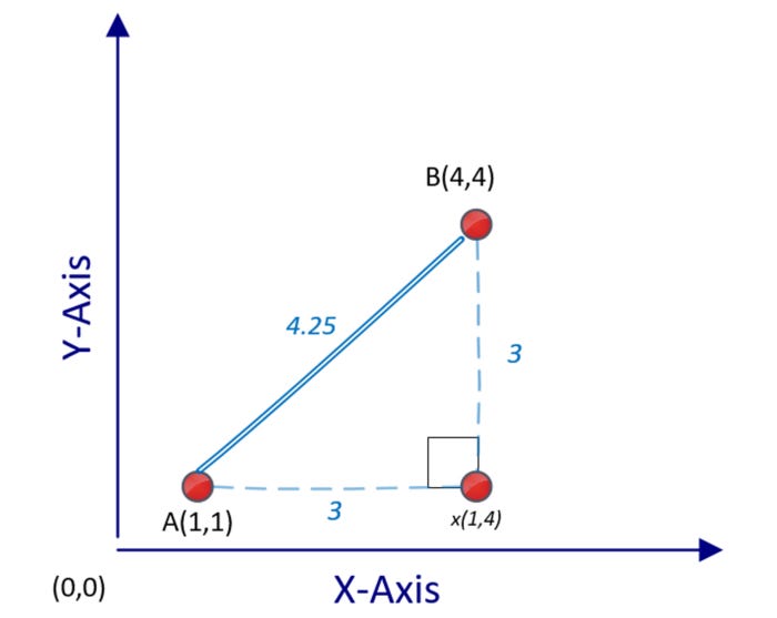
A and B’s distance d(A,B) can be calculated using Pythagorean formula:

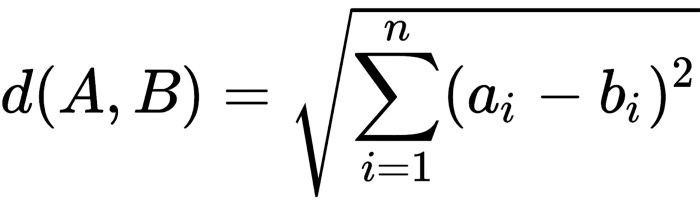
We are dealing with a two-dimensional problem space in this calculation. A distance between two points A and B in an n-dimensional problem space can be calculated as follows:
Manhattan distance
Using Euclidean distance to measure a shortest distance will not always indicate how similar or close two points are in many situations. As an example, if two data points represent locations on a map, then the actual distance between point A and point B is greater than the Euclidean distance calculated by ground transportation, such as a car or taxi. A Manhattan distance, which signifies the longest route between two points, is a better representation of the proximity of two points in the context of destination and source points that can be traveled to in a busy city. Here is a plot comparing Manhattan distance and Euclidean distance:
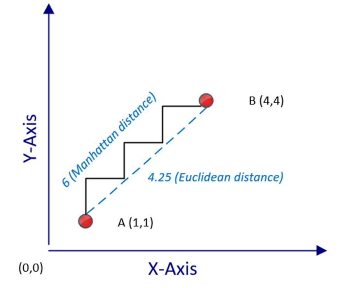
It is important to note that the Manhattan distance will always be greater than the corresponding Euclidean distance.
Cosine distance
High-dimensional space does not perform well for Euclidean and Manhattan distance measures. Cosine distance can be used to determine how close two data points are in a multidimensional problem space with many dimensions. In cosine distance measurements, two points are connected to a reference point by measuring the cosine angle. No matter what the dimensions of the data points are, the angle will be narrow if they are close together. The angle will be large if they are far apart, on the other hand:
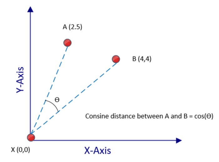
It is almost possible to consider textual data as a highly dimensional space. When dealing with textual data, the cosine distance measure is a good choice since it works well with spaces with h dimensions.
The cosine distance between A(2,5) and B(4.4) in the preceding figure is equal to the cosine of the angle between those two numbers. It is the origin — X(0,0) — that connects these points. There is no requirement that the origin must be the reference data point in a problem space.
Clustering algorithm based on K-means
In the k-means clustering algorithm, data points are clustered by computed means to find how close they are to each other. Due to its scalability and speed, it remains popular despite its simple clustering approach. Based on an iterative algorithm, k-means clustering moves the cluster centers until they represent the most representative data point of the cluster.
A very basic functionality required for clustering is missing from k-means algorithms. Specifically, the k-means algorithm cannot determine the number of clusters that are most appropriate for a given dataset. Depending on the number of natural groupings in a dataset, k, is the most appropriate number of clusters.
In order to maximize the performance of the algorithm, this omission is necessary in order to keep it as simple as possible. K-means can handle larger datasets because of this lean-and-mean design. It is assumed that k will be calculated by an external mechanism. Our best method for determining k will depend on the problem we are trying to solve. Depending on the clustering problem, k can be directly determined by the context of the clustering problem — for example, if we wanted to separate students into two clusters based on their data science and programming skills, then k would be two. It may not be obvious what the value of k is in some other problems. To determine which clusters are most appropriate for a given dataset, iterative trial-and-error procedures or heuristic-based algorithms will need to be used.
Clustering with k-means logic
K-means clustering is described in this section. We will examine them one by one.
The initialization process
Data points are grouped using a distance measure to determine their similarity or closeness through the k-means algorithm. Selecting the most appropriate distance measure is required before applying the k-means algorithm. Euclidean distance is the default distance measure. Moreover, if there are outliers in the dataset, then a mechanism must be devised for identifying them and removing them.
Algorithm steps for k-means
A k-means clustering algorithm consists of the following steps:
Step 1
It is decided how many clusters, k, are to be used.
Step 2
Among the data points, k points are randomly selected as cluster centers.
Step 3
The distance from each point in the problem space to each of the k cluster centers is iteratively computed using the selected distance measure. It may take some time to calculate 30,000 distances depending on the size of the dataset. If there are 10,000 points in the cluster and k = 3, for example, 30,000 distances need to be calculated.
Step 4
The nearest cluster center is assigned to each data point in the problem space.
Step 5
We have now assigned cluster centers to each of the data points in our problem space. As a random selection process was used to select the initial cluster centers, we are not yet done. Currently, we are using randomly selected cluster centers as centers of gravity. Using the means of the constituent data points of each cluster, we recalculate the cluster centers. The k-means algorithm gets its name from this step.
Step 6
When the cluster centers shift in step 5, we need to recompute each data point’s cluster assignment. We will repeat the compute-intensive step in step 3 to accomplish this. Upon satisfying our predetermined stop condition (for example, the number of maximum iterations), we are done if the cluster centers haven’t shifted.
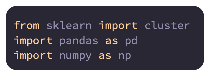
Using a two-dimensional problem space, the k-means algorithm produces the following result:
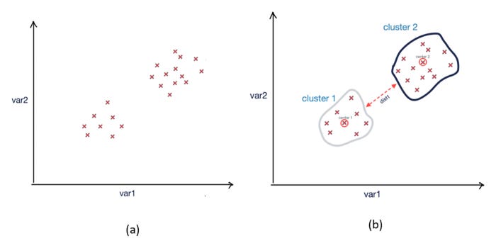
Resultant clusters after running k-means clustering; (a) Before clustering; (b) After clustering
There is a good level of differentiation between the two clusters created by k-means.
Condition of stop
When cluster centers stop shifting in step 5 of the k-means algorithm, it is considered to have reached its default stop condition. In a high-dimensional problem space, processing large datasets can take a long time for k-means algorithms, as with many other algorithms. It is also possible to explicitly define the stop condition before the algorithm converges, as follows:
If you specify a maximum execution time, you will be able to:
This is the stop condition: t>tmax, where t is the current execution time and tmax is the maximum execution time we have set.
Setting a maximum number of iterations will allow you to:
The algorithm is terminated if m>mmax, where m is the number of iterations currently in progress and mmax is the maximum number.
Algorithm coding for k-means
Python can be used to code the k-means algorithm as follows:
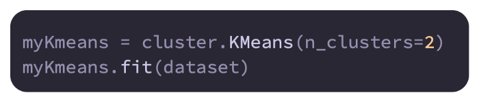
The first step in coding the k-means algorithm will be to import the necessary packages. For clustering using k-means, we are importing sklearn:
Let’s create a two-dimensional problem space, which will be used for k-means clustering, and place 20 data points within it:
With two clusters (k = 2), let’s call the fit functions and create the cluster:
We’ll create a variable called centroid that holds the location of the cluster’s center in an array. In our case, k = 2 means the array size is 2. We will also create a second variable called label to represent the clustering of the data points. This array will have a size of 20 since there are 20 data points:
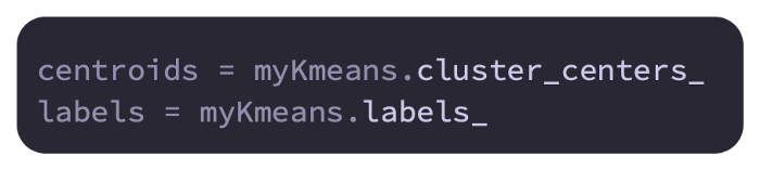
Here are the centroids and labels of these two arrays:
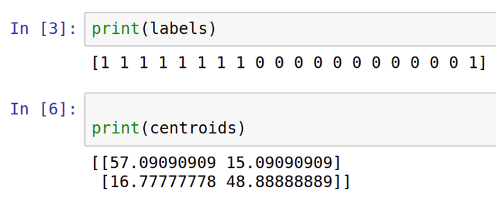
In the first array, cluster assignments are shown with each data point, while in the second array, cluster centers are displayed.
Using Matplotlib, plot the clusters as follows:
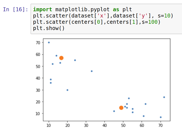
Based on the k-means algorithm, the larger dots on the plot represent centroids.
K-means clustering has limitations
As a simple and fast algorithm, k-means is designed to solve problems quickly. Due to its intentionally simple design, it has the following limitations:
K-means clustering has the biggest limitation of requiring a predetermined number of clusters.
Cluster centers are randomly assigned at the beginning. The algorithm can produce slightly different clusters every time it is run.
There is only one cluster assigned to each data point.
It is sensitive to outliers when using k-means clustering.
Clustering based on hierarchy
Clustering using k-means is a top-down approach since the algorithm starts from the cluster centers, which are the most relevant data points. In an alternative approach, we start the clustering algorithm from the bottom, rather than from the top. Each data point in the problem space is the bottom in this context. As data points progress toward the cluster centers, similar data points are grouped together. Hierarchical clustering algorithms use this alternative bottom-up approach, and this section discusses it.
Hierarchical clustering steps
A hierarchical clustering process involves the following steps:
In our problem space, we create separate clusters for each data point. It will start with 100 clusters if our problem space has 100 data points.
Those points that are closest to each other are grouped together.
In step 2, we check to see if the stop condition has been satisfied; if not, we repeat that step.
Dendrograms are clustered structures.
As shown in the following diagram, the height of the vertical lines determines the closeness of items in a dendrogram:
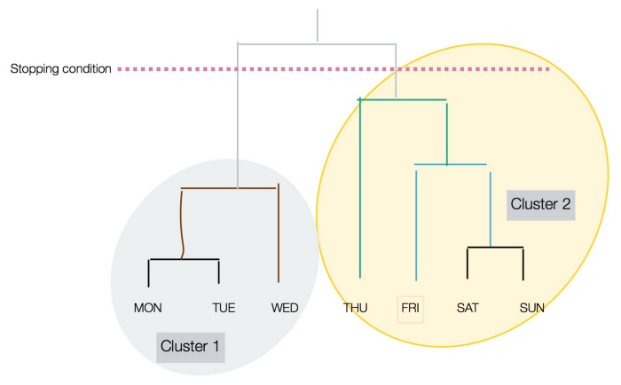
As you can see in the preceding figure, the stopping condition can be distinguished by a dotted line.
Algorithms for hierarchical clustering
Python hierarchical algorithms are easy to code:
In order to import AgglomerativeClustering from Sklearn.Cluster and the numpy and pandas packages, we will first import:
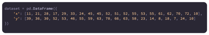
In a two-dimensional problem space, we will create 20 data points:
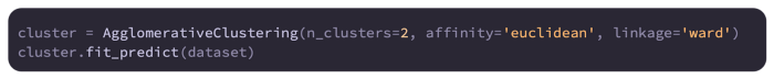
After specifying the hyperparameters, we create the hierarchical cluster. Our algorithm is actually processed using the fit_predict function:
To analyze the association between each data point and the two clusters, we can look at the following:
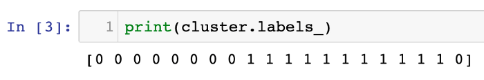
In both hierarchical and k-means algorithms, clusters are assigned similarly.
Cluster evaluation
Data points that belong to separate clusters should be distinguishable when clustering is done with good quality. Therefore, the following is implied:
There should be as much similarity as possible among the data points belonging to the same cluster.
Clusters should have as many data points as possible that are different from one another.
Clustering results can be evaluated by visualizing the clusters or by using mathematical methods that quantify cluster quality. Using silhouette analysis, you can compare the tightness and separation of clusters created by k-means. In the silhouette, points are plotted according to their proximity to each other in the neighboring clusters.
Each cluster is associated with a number between -0 and 1. Below is a table showing what these figures mean:
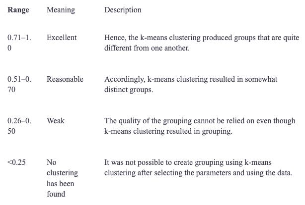
Throughout the problem space, each cluster will receive a separate score.
Clustering applications
Whenever the underlying pattern of a dataset needs to be revealed, clustering is used.
The following government use cases can benefit from clustering:
An analysis of crime hotspots
An analysis of demographics and social behavior
Clustering can be used in market research for the following purposes:
Segmentation of markets
Advertisements targeted at specific audiences
Organizing customers based on their characteristics
Stock-market trading data is also subject to principal component analysis (PCA) to remove noise.
Reduction of dimensions
A dimension in our problem space corresponds to each feature in our data. It is called dimensionality reduction when we reduce the number of features in our problem space in order to simplify it. One of two ways can be used:
In the context of the problem that we are trying to solve, selecting features that are important is key
One of the following algorithms can be used to combine two or more features in order to reduce dimensions:
Unsupervised linear machine learning algorithm PCA
A linear supervised machine learning algorithm called linear discriminant analysis (LDA)
A nonlinear algorithm for kernel principal component analysis
PCA is one of the most popular algorithms for dimensionality reduction.
Analyzing the principal components
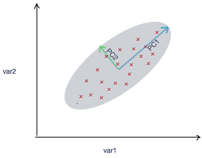
Unsupervised machine learning techniques, such as PCA, can be used to reduce dimensions by using linear transformations. The following figure shows two principle components, PC1 and PC2, which illustrate how the data points are spread out. The data points can be summarized with appropriate coefficients using PC1 and PC2:
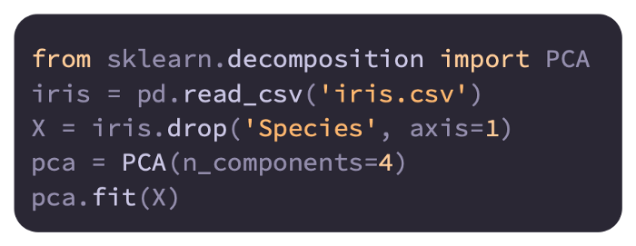
Here is a code example:
Our PCA model’s coefficients can now be printed:
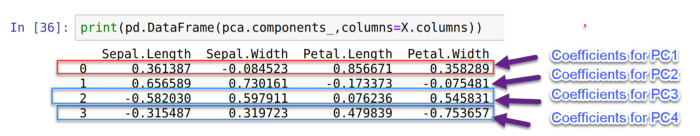
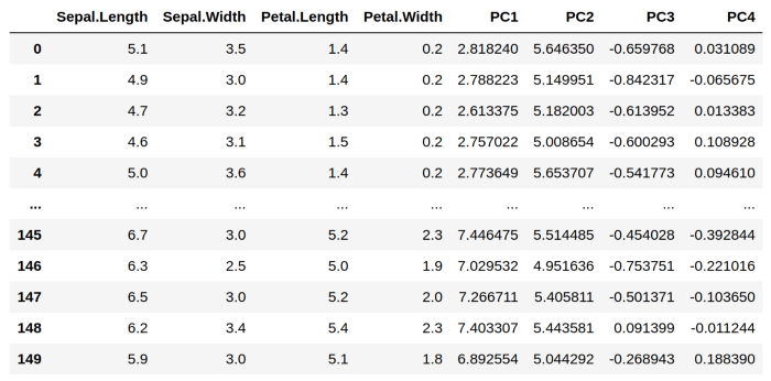
It is important to note that the original DataFrame consists of four features, Sepal.Length, Sepal.Width, Petal.Length, and Petal.Width. As shown in the preceding DataFrame, PC1, PC2, PC3, and PC4 have coefficients that can be used to replace the original four variables, namely PC1, PC2, and PC3.
Our input DataFrame X can be calculated based on these coefficients:
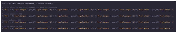
Here is X after the PCA components have been calculated:
Here is an example of PCA’s implications using the variance ratio:

According to the variance ratio, the following is true:
We can capture about 92.3% of the variance of the original variables by replacing the original four features with PC1. Due to the variance of the four original features, we will introduce some approximations.
We will capture an additional 5.3 % of the variance of the original variables if we replace the original four features with PC1 and PC2.
A further 0.017 % of the variance will be captured if PC1, PC2, and PC3 replace the original four features.
We will capture 100% of the variance of the original variables if we replace the original four features with four principal components (92.4 + 0.053 + 0.017 + 0.005), however it is pointless to replace four original features with four principal components since we did not reduce the dimensions at all.
PCA’s limitations
In addition to its limitations, PCA also has the following advantages:
Categorized variables cannot be analyzed with PCA because it is only applicable to continuous variables.
By simplifying the problem of dimensionality, PCA reduces accuracy while aggregating variables. Before using PCA, it is important to carefully consider this trade-off.
Rules of the association
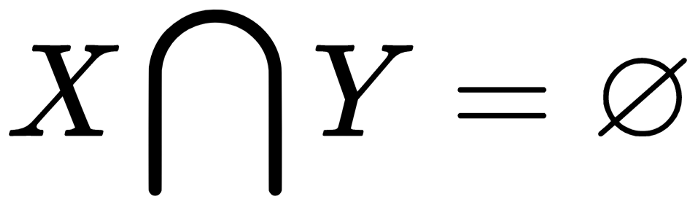
In various transactions, relationship items are described mathematically by association rules. To do this, it investigates the relationship between two sets of items in the form X ⇒ Y, where X ⊂ pie, Y ⊂ pie.
In addition, X and Y are nonoverlapping itemsets; which means that
.
The following are examples of association rules:
{helmet,balls}⇒ {bike}X and Y are [helmet,ball].Rule types
By running associative analysis algorithms on transaction datasets, a large number of rules will be generated. They are mostly useless. It is possible to classify rules into one of three types based on their potential to provide useful information:
Trivial
Inexplicable
Actionable
In this section, we will examine each type in more detail.
Trivial rules
There will be many rules generated from the large number of data points, but many of them will be useless since they sum up common knowledge about the business. Trivial rules are referred to as such. Despite the high level of confidence in trivial rules, they cannot be used to make data-driven decisions. There is no need to pay attention to trivial rules.
Trivial rules include the following:
Jumpers are likely to die if they jump from high-rise buildings.
The more you work, the better your exam results will be.
With a drop in temperature, heater sales increase
Highway accidents are more likely to occur when drivers exceed the speed limit.
Inexplicable rules
A rule that has no obvious explanation among those generated by the association rules algorithm is the trickiest to use. Remember that a rule is only useful if it can provide insight into a new pattern that eventually leads to a desired outcome. A mathematical formula that ends up exploring the pointless relationship between unrelated and independent events is inexplicable if that’s not the case, and we cannot explain why event X led to event Y.
Among the inexplicable rules are the following:
Exam results tend to be better for people wearing red shirts.
Theft is more likely to occur with green bicycles.
Diapers are also bought by people who buy pickles.
Actionable rules
The golden rule is to develop actionable rules. Businesses understand them and gain insights from them. By presenting actionable rules to an audience familiar with the business domain, we can discover possible causes for an event. For example, we may be able to determine where a product should be placed in a store based on current buying patterns. Users tend to buy items together, so they may suggest placing them together to maximize their sales.
An example of an actionable rule is as follows:
Users are more likely to purchase when ads are displayed on their social media accounts.
A suggestion for alternative ways to advertise a product is an actionable item
Sales are more likely to occur when there are more price points.
The price of one item may be raised while another is advertised in a sale.
