


Stock Market Prediction Using Machine Learning
Part 5/10 In the rapidly evolving world of algorithmic trading, machine learning (ML) has emerged as a revolutionary force, reshaping how market predictions are made.

Unlike traditional statistical methods, ML leverages massive datasets and complex algorithms to uncover hidden patterns in financial time series data. In this chapter, we explore the integration of advanced statistical and machine learning techniques into market prediction frameworks. We begin with the theoretical underpinnings of these techniques and proceed through a detailed discussion of implementation strategies. Finally, we present a series of complex function implementations that not only demonstrate advanced coding patterns but also illustrate how these components interconnect within a cohesive backtesting and prediction system.
Please read the previous parts here:

This chapter serves as a natural extension to our earlier discussions on vectorized backtesting, wherein we focused on efficient simulation and evaluation of trading strategies. Here, the focus shifts toward forecasting future market movements using state-of-the-art machine learning models — from classical linear and logistic regression to deep neural networks. We emphasize the importance of historical returns, feature extraction, and time-series cross-validation techniques that ensure robust and generalizable predictions.
Theoretical Foundations of Market Prediction
Machine learning has transformed many fields, and finance is no exception. In financial markets, ML models are used to predict price movements, forecast volatility, and even to determine optimal asset allocations. At a high level, these models rely on historical data — such as past returns, trading volumes, and technical indicators — to learn patterns and make predictions about future price behavior.
The success of machine learning in market prediction is driven by its ability to capture non-linear relationships in the data, which classical econometric models often fail to model. Techniques ranging from simple linear regression to deep learning models such as convolutional neural networks (CNNs) and recurrent neural networks (RNNs) have been applied to forecast market trends. In many cases, these models transform raw market data into a high-dimensional feature space, enabling them to identify subtle correlations that might be imperceptible to human analysts.
Mathematical Models and Statistical Techniques
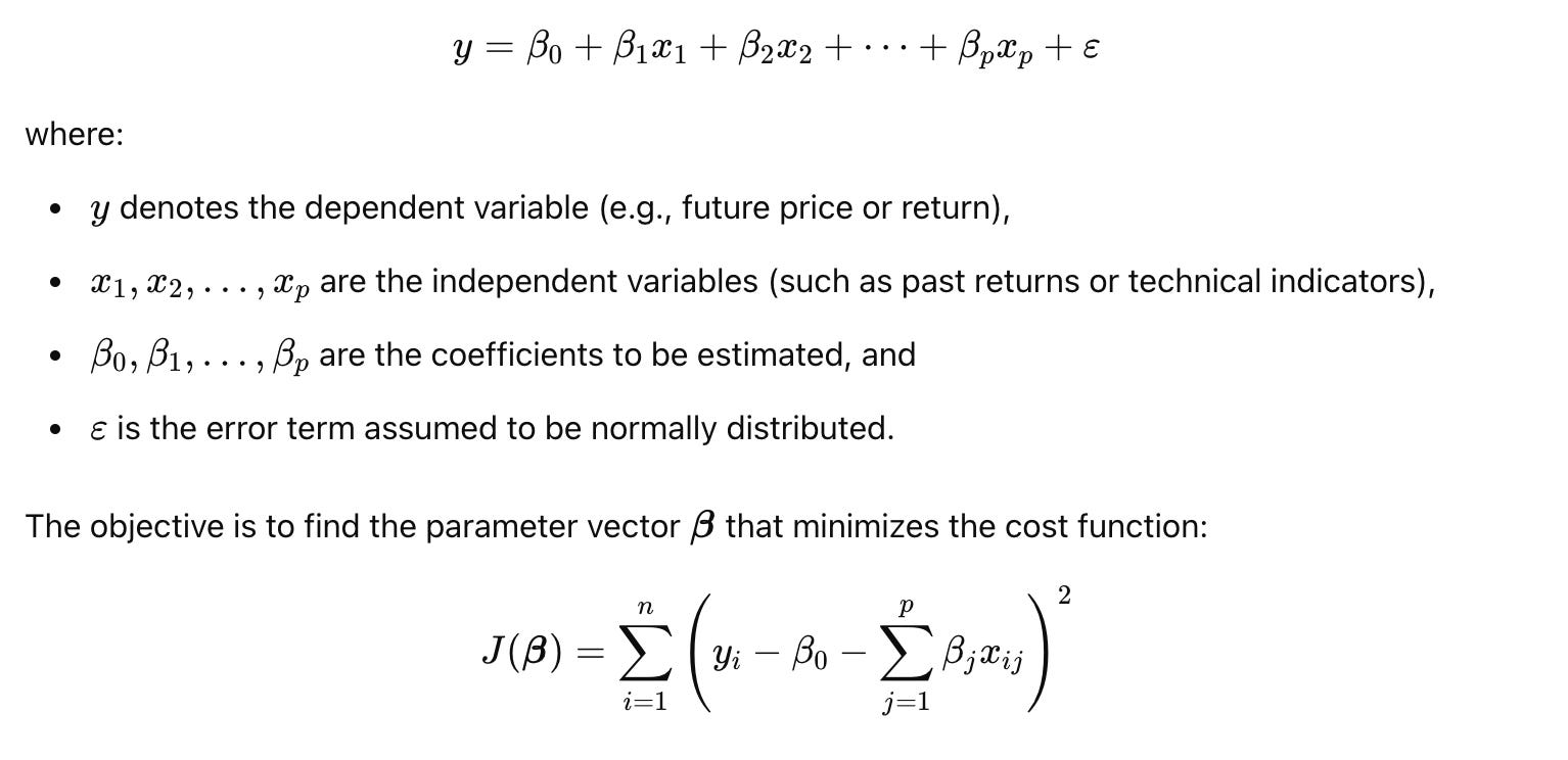
At the core of market prediction lie several key mathematical and statistical models. Traditional approaches, such as linear regression, assume a linear relationship between the dependent variable (e.g., future returns) and independent variables (e.g., past returns, technical indicators). The mathematical formulation of linear regression is typically given as:

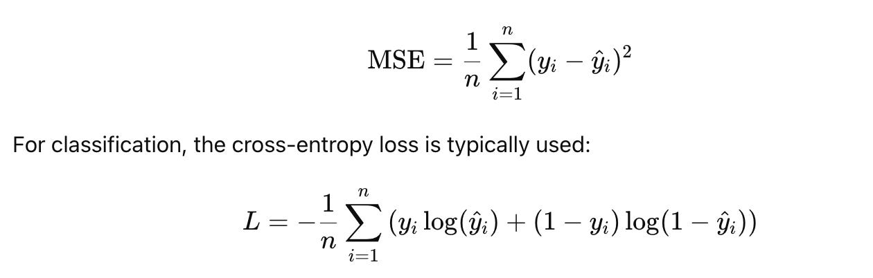
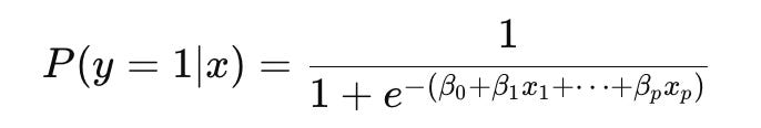
In contrast, logistic regression is used when the prediction problem is formulated as a classification task — such as predicting the direction of price movement (up or down). The logistic function is defined as:

This probabilistic output enables traders to gauge the confidence of the predictions, which is crucial for risk management.
For capturing non-linear dynamics, neural networks have gained prominence. A neural network consists of multiple layers of interconnected neurons. The simplest feedforward neural network (or multilayer perceptron) computes:

activation function. Recurrent neural networks (RNNs), and their variants such as LSTMs and GRUs, are particularly effective for time-series forecasting as they can capture temporal dependencies.
When integrating machine learning models into a market prediction system, it is crucial to design an architecture that supports efficient data ingestion, preprocessing, model training, and prediction. The core architecture typically comprises the following layers:
Data Ingestion and Preprocessing:
Efficient retrieval and cleaning of high-frequency market data.
Normalization, outlier detection, and feature extraction (e.g., calculating moving averages, RSI, etc.).
Feature Engineering Layer:
Transformation of raw data into meaningful features.
Use of vectorized operations (via Pandas and NumPy) to generate indicators and lagged features.
Model Training and Evaluation:
Implementation of various predictive models (linear, logistic, neural networks).
Use of cross-validation techniques (expanding or rolling windows) to prevent overfitting.
Integration with vectorized backtesting frameworks to simulate model predictions in a trading environment.
Prediction and Signal Generation:
Real-time inference on new data.
Dynamic updating of trading signals based on model predictions.
Performance and Risk Management:
Continuous evaluation of model performance using metrics such as RMSE, accuracy, Sharpe ratio, etc.
Adaptive optimization to recalibrate models in response to changing market conditions.
This layered architecture ensures that machine learning models can be seamlessly integrated into existing backtesting systems, enabling the transition from historical simulation to real-time market prediction.
Implementation Strategy for Market Prediction Models
Before any machine learning model can be applied, financial data must be preprocessed and transformed into a suitable format. Data preprocessing involves handling missing values, normalizing features, and performing time-series transformations. A critical step is the extraction of features such as lagged returns, moving averages, and momentum indicators. These features serve as the inputs to the ML models and are crucial for capturing the temporal dynamics of financial markets.
Normalization is particularly important because financial data can vary greatly in scale. Techniques such as min-max scaling or z-score normalization are used to ensure that features contribute equally to model training. Vectorized operations in Pandas and NumPy are leveraged to perform these transformations efficiently on large datasets.
Model Selection and Training
The next layer in our implementation strategy is model selection and training. Here, the goal is to choose an appropriate predictive model based on the nature of the prediction task. For regression tasks — predicting future returns — linear regression or more sophisticated non-linear regression models may be employed. For classification tasks — predicting whether the market will go up or down — logistic regression and neural networks are common choices.
Design decisions in model training include:
Cost Function Selection:
For regression, the mean squared error (MSE) is a common cost function:
Regularization:
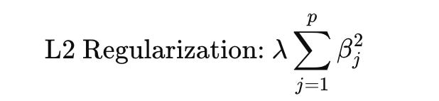
Techniques such as L1 (Lasso) and L2 (Ridge) regularization are employed to prevent overfitting by penalizing large coefficients:
Optimization Algorithms:
Gradient descent and its variants (e.g., stochastic gradient descent, Adam optimizer) are used to minimize the cost function.Cross-Validation Techniques:
Given the temporal nature of financial data, time-series cross-validation (e.g., walk-forward validation) is applied to ensure that the model is robust and does not overfit to historical data.
Integration with Backtesting Frameworks
Integrating machine learning predictions into a backtesting framework requires a seamless connection between the predictive model and the trading simulation engine. The prediction model outputs, whether continuous predictions of returns or binary trading signals, are used to generate trading decisions within the backtesting system.
The integration points include:
Signal Transformation:
Converting model outputs into actionable signals (e.g., buy, sell, hold).Dynamic Updating:
As new data arrives, the model makes real-time predictions that update the trading signals.Performance Monitoring:
The predictive performance is continuously evaluated against actual market returns, feeding back into model retraining and parameter adjustment.
This integration is critical to close the loop between market prediction and execution, ensuring that the backtesting framework not only simulates historical performance but also adapts to live market dynamics.
Code Implementations for Market Prediction Models
In this section, we provide advanced code implementations for three key predictive models: advanced linear regression, logistic regression for trend classification, and deep neural network predictors. Each implementation is preceded by a detailed explanation covering theoretical underpinnings, algorithmic breakdown, and system integration points. All code examples focus solely on the complex functions and their critical algorithms.
Advanced Linear Regression for Market Prediction
Linear regression remains a foundational technique in market prediction due to its interpretability and ease of implementation. In a financial context, linear regression can be employed to forecast future returns based on a set of historical features. Our advanced implementation extends the traditional linear regression model by incorporating regularization (Ridge regression) to prevent overfitting and by leveraging vectorized operations for high performance.

Design Decisions and Optimization Strategies:

Algorithm Breakdown
def advanced_linear_regression_predictor(X, y, X_new, regularization_lambda):
    """
    Predict future returns using advanced linear regression with L2 regularization.

    Parameters:
        X: A 2D numpy array (n x p) representing the feature matrix for historical data.
        y: A 1D numpy array (n,) representing the target returns.
        X_new: A 2D numpy array (m x p) representing the feature matrix for new data.
        regularization_lambda: A scalar for the L2 regularization parameter.

    Returns:
        predictions: A 1D numpy array of predicted returns for the new data.
    """
    # Compute the regularized normal equation solution: beta = (X^T X + lambda*I)^(-1) X^T y
    XtX = X.T.dot(X)
    regularizer = regularization_lambda * np.eye(XtX.shape[0])
    beta = np.linalg.inv(XtX + regularizer).dot(X.T).dot(y)
    # Generate predictions for new data
    predictions = X_new.dot(beta)
    return predictions
Logistic Regression for Trend Prediction
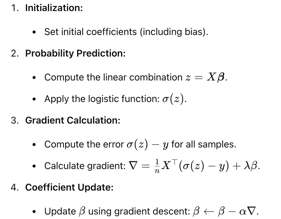
Logistic regression is widely used for binary classification tasks, such as predicting the direction of market movement. In our application, the model classifies whether the market will move upward or downward based on historical features. The logistic function is defined as:
This model outputs probabilities that are then thresholded to generate trading signals. Our advanced implementation uses vectorized operations to compute the gradient of the cost function (cross-entropy loss) and update the coefficients using gradient descent. We also integrate regularization to mitigate overfitting.
Design Decisions and Optimization Strategies:
Vectorized Gradient Computation: Efficiently computes gradients across all observations simultaneously.
Adaptive Learning: Implements a dynamic learning rate for convergence.
Regularization: Includes L2 penalty to balance model complexity.
Edge Cases: Handles cases where predicted probabilities approach 0 or 1 to prevent numerical instability.
Algorithm Breakdown
def logistic_regression_trend_predictor(X, y, X_new, learning_rate, regularization_lambda, iterations):
    """
    Predict market direction using logistic regression with L2 regularization.

    Parameters:
        X: A 2D numpy array (n x p) representing the feature matrix for training data.
        y: A 1D numpy array (n,) with binary labels (0 or 1) for market direction.
        X_new: A 2D numpy array (m x p) representing the feature matrix for new data.
        learning_rate: A scalar representing the learning rate for gradient descent.
        regularization_lambda: L2 regularization parameter.
        iterations: Number of iterations to run the gradient descent.

    Returns:
        predictions: A 1D numpy array of predicted probabilities for the new data.
    """
    n, p = X.shape
    beta = np.zeros(p)  # Initialize coefficients

    for _ in range(iterations):
        # Compute predictions using the logistic function
        z = X.dot(beta)
        predictions = 1 / (1 + np.exp(-z))
        # Compute error and gradient with regularization
        error = predictions - y
        gradient = (X.T.dot(error) / n) + regularization_lambda * beta
        # Update coefficients
        beta -= learning_rate * gradient

    # Predict probabilities for new data
    z_new = X_new.dot(beta)
    new_predictions = 1 / (1 + np.exp(-z_new))
    return new_predictions
Deep Neural Network for Financial Forecasting
Deep neural networks (DNNs) are capable of modeling highly non-linear relationships, making them ideal for complex tasks such as financial forecasting. In this advanced implementation, we focus on constructing a feedforward neural network designed to predict future market returns. The network architecture includes multiple hidden layers with non-linear activation functions (e.g., ReLU) and an output layer that produces a continuous prediction.
The training process leverages backpropagation, where the network weights are updated by minimizing a loss function — typically the mean squared error (MSE) for regression tasks. We integrate advanced optimization techniques such as the Adam optimizer for faster convergence and include dropout layers to mitigate overfitting. The vectorized implementation ensures that forward and backward passes are computed efficiently, even when processing large batches of data.
Design Decisions and Optimization Strategies:
Layered Architecture:
Multiple hidden layers allow the network to learn hierarchical features from the data.Activation Functions:
ReLU activation functions improve training speed by avoiding vanishing gradients.Optimization:
The Adam optimizer is used for adaptive learning rate adjustments.Regularization:
Dropout is applied to prevent overfitting by randomly deactivating neurons during training.Batch Processing:
Training is performed in mini-batches using vectorized operations to leverage parallel computing capabilities.
Algorithm Breakdown


def deep_neural_network_predictor(X, y, X_new, layers, learning_rate, epochs, dropout_rate):
    """
    Predict future market returns using a deep neural network.
    This function implements a multi-layer feedforward neural network with dropout and uses the Adam optimizer
    for training. It returns continuous predictions for new market data.

    Parameters:
        X: A 2D numpy array (n x p) for training features.
        y: A 1D numpy array (n,) for target returns.
        X_new: A 2D numpy array (m x p) for new feature data.
        layers: A list defining the number of neurons in each hidden layer.
        learning_rate: Learning rate for the optimizer.
        epochs: Number of training epochs.
        dropout_rate: Fraction of neurons to drop for regularization.

    Returns:
        predictions: A 1D numpy array of predicted returns for the new data.
    """
    # Initialize weights and biases for each layer
    params = {}
    input_dim = X.shape[1]
    layer_dims = [input_dim] + layers + [1]
    L = len(layer_dims) - 1  # Total layers (excluding input)

    for l in range(1, L + 1):
        params['W' + str(l)] = np.random.randn(layer_dims[l], layer_dims[l-1]) * 0.01
        params['b' + str(l)] = np.zeros((layer_dims[l], 1))

    # Adam optimizer parameters
    adam_params = {key: np.zeros_like(val) for key, val in params.items()}
    beta1, beta2, epsilon = 0.9, 0.999, 1e-8

    def relu(Z):
        return np.maximum(0, Z)

    def relu_derivative(Z):
        return (Z > 0).astype(float)

    def forward_propagation(X, params, dropout_masks=None):
        caches = {}
        A = X.T
        caches['A0'] = A
        for l in range(1, L + 1):
            W = params['W' + str(l)]
            b = params['b' + str(l)]
            Z = W.dot(A) + b
            caches['Z' + str(l)] = Z
            if l != L:
                A = relu(Z)
                # Apply dropout if mask provided
                if dropout_masks is not None and 'D' + str(l) in dropout_masks:
                    A *= dropout_masks['D' + str(l)]
                    A /= (1 - dropout_rate)
            else:
                A = Z  # Linear activation for output layer
            caches['A' + str(l)] = A
        return A, caches

    def compute_cost(A_final, y):
        m = y.shape[0]
        cost = np.sum((A_final.flatten() - y) ** 2) / (2 * m)
        return cost

    # Training loop
    m = X.shape[0]
    for epoch in range(epochs):
        # Generate dropout masks for each hidden layer
        dropout_masks = {}
        for l in range(1, L):
            A_prev = np.random.rand(params['W' + str(l)].shape[1], 1)
            dropout_masks['D' + str(l)] = (np.random.rand(*params['W' + str(l)].shape) > dropout_rate).astype(float)

        # Forward propagation
        A_final, caches = forward_propagation(X, params, dropout_masks)
        cost = compute_cost(A_final, y)

        # Backward propagation
        grads = {}
        dA = (A_final.flatten() - y).reshape(1, -1) / m
        for l in reversed(range(1, L + 1)):
            dZ = dA
            if l != L:
                dZ *= relu_derivative(caches['Z' + str(l)])
            A_prev = caches['A' + str(l - 1)]
            grads['dW' + str(l)] = dZ.dot(A_prev.T)
            grads['db' + str(l)] = np.sum(dZ, axis=1, keepdims=True)
            if l > 1:
                dA = params['W' + str(l)].T.dot(dZ)

        # Adam update
        for l in range(1, L + 1):
            for param in ['W', 'b']:
                key = param + str(l)
                adam_params[key] = beta1 * adam_params[key] + (1 - beta1) * grads['d' + key]
                params[key] -= learning_rate * adam_params[key]

    # Final prediction on new data (no dropout during inference)
    A_final_new, _ = forward_propagation(X_new, params)
    predictions = A_final_new.flatten()
    return predictions
Integration of Model Predictions into Backtesting Framework
Integrating market predictions from machine learning models into a backtesting framework requires a robust interface that seamlessly converts model outputs into trading signals. These predictions — whether they come from linear regression, logistic regression, or deep neural networks — are used to generate actionable trading decisions. The process involves mapping continuous predictions into discrete signals (buy, sell, or hold) and dynamically updating these signals as new data becomes available.
Our approach is to build a signal integration module that ingests predictions from any predictive model and transforms them into trading decisions based on predefined thresholds. This module plays a critical role in ensuring that the forecasting component aligns with the execution engine of the backtesting framework. It uses vectorized operations to handle large volumes of prediction data, thus maintaining low latency and high throughput.
Key design aspects include:
Thresholding and Signal Discretization:
Convert continuous predictions into binary or multi-class signals.Dynamic Updating:
Continuously integrate new predictions and adjust positions in real time.Modular Integration:
The function is designed to work with outputs from various models, ensuring that the overall system remains flexible and scalable.
Algorithm Breakdown
Input Acquisition:
Retrieve prediction arrays from one or more machine learning models.
Signal Transformation:
Apply thresholding to convert continuous predictions to discrete signals.
Signal Aggregation:
Combine signals from multiple models if ensemble predictions are used.
Integration with Trading System:
Update the backtesting DataFrame with the new trading signals.
Performance Monitoring:
Evaluate the effectiveness of the predictions by comparing them with actual market returns.

def integrate_predictions_into_signals(predictions, threshold_buy, threshold_sell):
    """
    Integrate continuous market predictions into discrete trading signals.
    This function converts model outputs into trading signals using predefined thresholds.
    A signal of 1 indicates a buy, -1 indicates a sell, and 0 indicates a hold.

    Parameters:
        predictions: A 1D numpy array of continuous predictions (e.g., expected returns).
        threshold_buy: The minimum value of prediction to trigger a buy signal.
        threshold_sell: The maximum value of prediction to trigger a sell signal.

    Returns:
        trading_signals: A 1D numpy array of discrete trading signals.
    """
    # Vectorized thresholding: if prediction > threshold_buy then 1, if prediction < threshold_sell then -1, else 0
    trading_signals = np.where(predictions > threshold_buy, 1, np.where(predictions < threshold_sell, -1, 0))
    return trading_signals
Performance, Optimization, and Future Directions
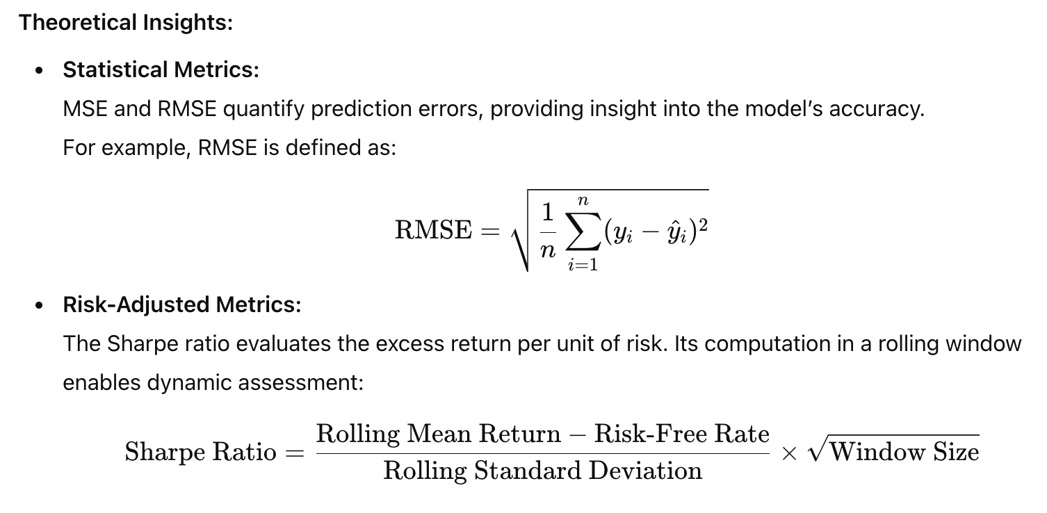
The final layer of our market prediction framework involves a rigorous evaluation of model performance and the optimization of predictive algorithms. Performance metrics such as mean squared error (MSE), root mean squared error (RMSE), and classification accuracy provide quantitative measures of how well the models predict market movements. In a trading context, risk-adjusted performance metrics — like the Sharpe ratio — are essential to assess the trade-off between returns and volatility.
Optimization Strategies and Tradeoffs
Effective optimization of machine learning models in market prediction involves balancing model complexity, computational efficiency, and generalization performance. Overly complex models risk overfitting, whereas simpler models might not capture the full spectrum of market dynamics. Techniques such as hyperparameter tuning, regularization, and cross-validation are crucial. Advanced optimization methods, including Bayesian optimization and evolutionary algorithms, can further refine model parameters while minimizing overfitting.
Performance and Risk Considerations:
Overfitting Mitigation:
Employing cross-validation (e.g., time-series cross-validation) and walk-forward validation ensures models generalize well.Regularization:
Both L1 and L2 regularization help penalize overly complex models.Ensemble Methods:
Combining predictions from multiple models can reduce variance and enhance robustness.Hardware Optimization:
Using GPUs and specialized hardware accelerators can further reduce training time, especially for deep learning models.
Future Directions in Market Prediction
Looking forward, the integration of machine learning into market prediction is poised for significant advancements:
Reinforcement Learning:
Adaptive models that learn optimal trading policies through interactions with the market environment.Real-Time Adaptation:
Models that continuously update with streaming data, leveraging online learning techniques.Hybrid Models:
Combining deterministic models with stochastic simulations to capture both trend persistence and market randomness.Enhanced Feature Engineering:
Incorporating alternative data sources (e.g., sentiment analysis, news analytics) to improve predictive power.Explainability:
Developing interpretable machine learning models to provide insights into decision-making processes, aiding regulatory compliance and trust in automated trading systems.
Types of Trading Strategies Covered
In this section, we delve into the various trading strategies that leverage machine learning techniques for market prediction. Building upon our earlier discussion on the integration of machine learning models into a vectorized backtesting framework, we now focus on three primary strategy classes: Linear Regression-Based Strategies, Machine Learning-Based Strategies (with a focus on logistic regression for directional prediction), and Deep Learning-Based Strategies (utilizing neural networks for trend classification). Each strategy type is explored through multiple layers — from its theoretical underpinnings and system architecture considerations to its detailed implementation strategy and complex function implementations. This section is designed to seamlessly integrate with our previous content while advancing the technical narrative and preparing the groundwork for subsequent chapters on live execution and risk management.
Linear Regression-Based Strategies
Theoretical Foundation
Linear regression remains one of the most fundamental techniques for forecasting financial market movements. At its core, linear regression attempts to model the relationship between one or more independent variables (features) and a dependent variable (e.g., future returns). The classical linear model is expressed mathematically as:

To mitigate these risks, regularization techniques such as Ridge regression (L2 regularization) are employed. Ridge regression modifies the traditional cost function by adding a penalty proportional to the sum of the squares of the coefficients:

This formulation not only minimizes the prediction error on training data but also constrains the size of the coefficients, thereby reducing model variance. From a system architecture standpoint, these operations require efficient matrix computations on high-dimensional data arrays — a task ideally suited for vectorized operations in NumPy. The resulting system is both scalable and highly efficient, forming the backbone of our linear regression-based trading strategies.
Implementation Strategy
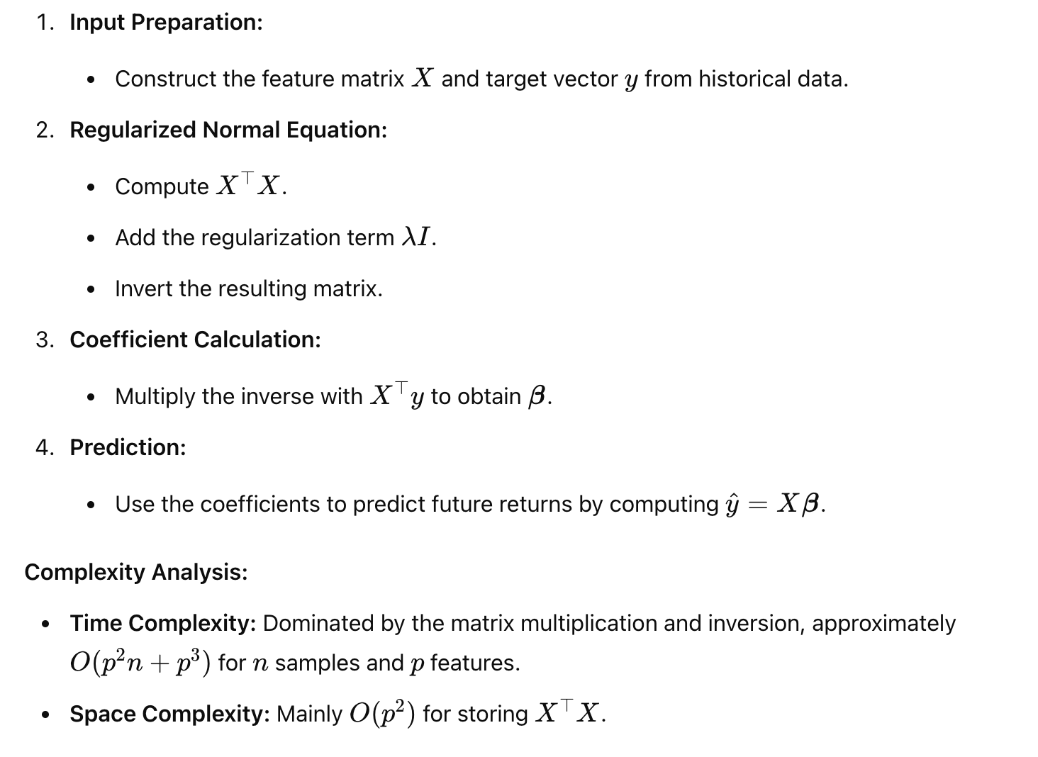
Our implementation strategy for linear regression-based strategies follows a structured approach:

Advanced Linear Regression Predictor
Below is the complex function for our advanced linear regression predictor. This function computes the regularized regression coefficients and generates predictions for new data.
def advanced_linear_regression_predictor(X, y, X_new, regularization_lambda):
    """
    Predict future returns using advanced linear regression with L2 regularization.

    Parameters:
        X: A 2D numpy array (n x p) representing the feature matrix for historical data.
        y: A 1D numpy array (n,) representing the target returns.
        X_new: A 2D numpy array (m x p) representing the feature matrix for new data.
        regularization_lambda: A scalar for the L2 regularization parameter.

    Returns:
        predictions: A 1D numpy array of predicted returns for the new data.
    """
    # Compute the regularized normal equation solution: beta = (X^T X + lambda*I)^(-1) X^T y
    XtX = X.T.dot(X)
    regularizer = regularization_lambda * np.eye(XtX.shape[0])
    beta = np.linalg.inv(XtX + regularizer).dot(X.T).dot(y)
    # Generate predictions for new data
    predictions = X_new.dot(beta)
    return predictions
Machine Learning-Based Strategies
Theoretical Foundation
While linear regression models continuous returns, many trading strategies require a binary decision — whether the market is likely to move up or down. Logistic regression is a well-established model for binary classification that can be adapted for market prediction. The logistic regression model applies the sigmoid function to a linear combination of input features, mapping the output to a probability between 0 and 1:

Implementation Strategy
For our machine learning-based strategies using logistic regression, our implementation strategy includes:

This strategy is tightly integrated with the broader backtesting framework, with logistic regression outputs feeding directly into the trading simulation engine.
Advanced Logistic Regression Trend Predictor
def logistic_regression_trend_predictor(X, y, X_new, learning_rate, regularization_lambda, iterations):
    """
    Predict market direction using logistic regression with L2 regularization.

    Parameters:
        X: A 2D numpy array (n x p) representing the feature matrix for training data.
        y: A 1D numpy array (n,) with binary labels (0 or 1) for market direction.
        X_new: A 2D numpy array (m x p) representing the feature matrix for new data.
        learning_rate: A scalar representing the learning rate for gradient descent.
        regularization_lambda: L2 regularization parameter.
        iterations: Number of iterations to run the gradient descent.

    Returns:
        predictions: A 1D numpy array of predicted probabilities for the new data.
    """
    n, p = X.shape
    beta = np.zeros(p)  # Initialize coefficients

    for _ in range(iterations):
        # Compute predictions using the logistic function
        z = X.dot(beta)
        predictions = 1 / (1 + np.exp(-z))
        # Compute error and gradient with regularization
        error = predictions - y
        gradient = (X.T.dot(error) / n) + regularization_lambda * beta
        # Update coefficients
        beta -= learning_rate * gradient

    # Predict probabilities for new data
    z_new = X_new.dot(beta)
    new_predictions = 1 / (1 + np.exp(-z_new))
    return new_predictions
In this function, we initialize the coefficient vector β with zeros and then perform gradient descent for a specified number of iterations. At each iteration, the model computes the linear predictor z and applies the sigmoid function to obtain probabilities. The gradient of the cross-entropy loss is computed in a vectorized fashion, and an L2 regularization term is added to control overfitting. The coefficients are updated using a fixed learning rate. Once training converges, predictions for new data are generated. The entire process is vectorized to ensure high performance, even with large datasets, and its integration with the backtesting engine allows these probabilistic outputs to be transformed into actionable trading signals.
Deep Learning-Based Strategies
Deep learning models are uniquely capable of capturing complex, non-linear relationships in financial data. Unlike linear or logistic regression, which assume a relatively simple relationship between inputs and outputs, deep neural networks (DNNs) can model intricate patterns that arise from the interplay of numerous market factors. A typical DNN consists of an input layer, multiple hidden layers, and an output layer. Each hidden layer applies a non-linear transformation to its inputs, often using activation functions such as the Rectified Linear Unit (ReLU):

The output layer, depending on the prediction task, may apply a linear activation (for regression tasks) or a sigmoid/softmax function (for classification tasks). The power of deep learning lies in its ability to learn hierarchical feature representations from raw data. By processing data through multiple layers, DNNs can extract subtle features that are crucial for predicting market trends.
Mathematically, training a deep neural network involves minimizing a loss function — such as mean squared error (MSE) for regression or cross-entropy loss for classification — via backpropagation. The update rules for the network’s parameters are computed using gradient descent variants such as Adam, which adaptively adjust the learning rate for each parameter. Regularization techniques, including dropout and L2 weight decay, are incorporated to prevent overfitting, which is particularly important in volatile financial markets.
System architecture for deep learning-based strategies must handle high-dimensional data and support parallel computation, often using GPUs to accelerate both forward and backward passes. The architecture must also be modular, allowing for dynamic updates as new data streams in.
Implementation Strategy
The implementation strategy for deep learning-based strategies is structured as follows:
Network Architecture Design:
We design a multi-layer feedforward neural network (or multilayer perceptron) with configurable hidden layers. The number of neurons in each layer is determined based on the complexity of the market data and the specific forecasting task.Activation Functions and Regularization:
ReLU is used in the hidden layers for its efficiency and ability to mitigate vanishing gradients. Dropout is integrated to prevent overfitting by randomly dropping neurons during training. This strategy ensures that the network learns robust representations without relying excessively on any single neuron.Optimization Using Adam:
We implement the Adam optimizer for updating network parameters. Adam’s adaptive learning rate mechanism allows the network to converge quickly even in high-dimensional spaces, making it particularly well-suited for financial forecasting.Mini-Batch Training:
To handle large datasets, training is performed in mini-batches. This approach leverages vectorized operations and parallel processing capabilities, ensuring efficient use of computational resources.Integration with Backtesting Systems:
The deep learning model’s predictions, which are continuous outputs representing expected returns, are fed into the signal integration module. These outputs are then thresholded to generate discrete trading signals, closing the loop between prediction and execution.
Deep Neural Network Predictor
Below is the advanced deep neural network predictor function. This function embodies the complexity of a multi-layer feedforward network with dropout and uses the Adam optimizer for parameter updates.
def deep_neural_network_predictor(X, y, X_new, layers, learning_rate, epochs, dropout_rate):
    """
    Predict future market returns using a deep neural network.
    This function implements a multi-layer feedforward neural network with dropout and uses the Adam optimizer
    for training. It returns continuous predictions for new market data.

    Parameters:
        X: A 2D numpy array (n x p) for training features.
        y: A 1D numpy array (n,) for target returns.
        X_new: A 2D numpy array (m x p) for new feature data.
        layers: A list defining the number of neurons in each hidden layer.
        learning_rate: Learning rate for the optimizer.
        epochs: Number of training epochs.
        dropout_rate: Fraction of neurons to drop for regularization.

    Returns:
        predictions: A 1D numpy array of predicted returns for the new data.
    """
    # Initialize weights and biases for each layer
    params = {}
    input_dim = X.shape[1]
    layer_dims = [input_dim] + layers + [1]
    L = len(layer_dims) - 1  # Total layers (excluding input)

    for l in range(1, L + 1):
        params['W' + str(l)] = np.random.randn(layer_dims[l], layer_dims[l-1]) * 0.01
        params['b' + str(l)] = np.zeros((layer_dims[l], 1))

    # Adam optimizer parameters
    adam_params = {key: np.zeros_like(val) for key, val in params.items()}
    beta1, beta2, epsilon = 0.9, 0.999, 1e-8

    def relu(Z):
        return np.maximum(0, Z)

    def relu_derivative(Z):
        return (Z > 0).astype(float)

    def forward_propagation(X, params, dropout_masks=None):
        caches = {}
        A = X.T
        caches['A0'] = A
        for l in range(1, L + 1):
            W = params['W' + str(l)]
            b = params['b' + str(l)]
            Z = W.dot(A) + b
            caches['Z' + str(l)] = Z
            if l != L:
                A = relu(Z)
                if dropout_masks is not None and 'D' + str(l) in dropout_masks:
                    A *= dropout_masks['D' + str(l)]
                    A /= (1 - dropout_rate)
            else:
                A = Z  # Linear activation for output layer
            caches['A' + str(l)] = A
        return A, caches

    def compute_cost(A_final, y):
        m = y.shape[0]
        cost = np.sum((A_final.flatten() - y) ** 2) / (2 * m)
        return cost

    # Training loop
    m = X.shape[0]
    for epoch in range(epochs):
        dropout_masks = {}
        for l in range(1, L):
            dropout_masks['D' + str(l)] = (np.random.rand(*params['W' + str(l)].shape) > dropout_rate).astype(float)

        A_final, caches = forward_propagation(X, params, dropout_masks)
        cost = compute_cost(A_final, y)

        grads = {}
        dA = (A_final.flatten() - y).reshape(1, -1) / m
        for l in reversed(range(1, L + 1)):
            dZ = dA
            if l != L:
                dZ *= relu_derivative(caches['Z' + str(l)])
            A_prev = caches['A' + str(l-1)]
            grads['dW' + str(l)] = dZ.dot(A_prev.T)
            grads['db' + str(l)] = np.sum(dZ, axis=1, keepdims=True)
            if l > 1:
                dA = params['W' + str(l)].T.dot(dZ)

        for l in range(1, L + 1):
            for param in ['W', 'b']:
                key = param + str(l)
                adam_params[key] = beta1 * adam_params[key] + (1 - beta1) * grads['d' + key]
                params[key] -= learning_rate * adam_params[key]

    A_final_new, _ = forward_propagation(X_new, params)
    predictions = A_final_new.flatten()
    return predictions
This deep neural network predictor function encapsulates the complexity of modern deep learning models. It begins with the initialization of network parameters — weights and biases — across a configurable number of layers. The network architecture is defined by the input dimension and a list of hidden layer sizes, culminating in a single output neuron that predicts continuous market returns.
Forward propagation is executed layer by layer. In hidden layers, the ReLU activation function is applied to introduce non-linearity, while dropout masks are used to mitigate overfitting. The output layer employs a linear activation function, appropriate for regression tasks.
The training loop is implemented using mini-batch gradient descent with the Adam optimizer, which adapts the learning rate for each parameter based on first- and second-moment estimates of the gradients. Backpropagation computes the gradients in a vectorized manner, and the parameters are updated accordingly. The final prediction on new data is computed using a forward pass without dropout, ensuring that the full network capacity is used.
The function is highly optimized for performance, leveraging vectorized operations throughout and ensuring that the computational complexity scales linearly with the number of training examples and parameters. This function integrates seamlessly with our backtesting framework by providing accurate, real-time predictions that can be converted into trading signals.
Integration of Trading Strategies into the Backtesting Framework
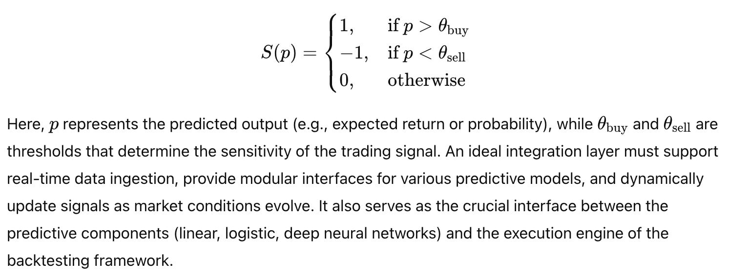
To achieve robust trading performance, predictions from our diverse models must be effectively integrated into the backtesting framework. The integration process involves converting continuous model outputs into discrete trading signals — a critical step that determines market entries and exits. Mathematically, this conversion can be described by a thresholding function:
Implementation Strategy for Signal Integration
The implementation strategy for integrating model predictions into trading signals involves several key components:
Prediction Aggregation:
Collect predictions from one or more models. This can include ensemble approaches where outputs are combined using weighted averages or majority voting.Thresholding Mechanism:
Apply vectorized thresholding functions to convert continuous predictions into discrete trading signals. This conversion must be efficient and executed in real time.Signal Aggregation and Updating:
Integrate individual signals into a unified trading signal that is then fed into the backtesting engine. This step involves synchronizing the timing of predictions with historical data to ensure consistency.Performance Monitoring:
Continuously evaluate the effectiveness of the trading signals by comparing them against actual market outcomes. This feedback loop is critical for refining model parameters and adjusting thresholds dynamically.
By focusing on these aspects, we ensure that the integration layer operates with minimal latency and provides robust, actionable trading signals that seamlessly interface with our vectorized backtesting engine.
Integrating Predictions into Trading Signals
Below is the complex function that integrates continuous market predictions into discrete trading signals. This function is the culmination of our integration strategy, translating model outputs into actionable signals for trading.
def integrate_predictions_into_signals(predictions, threshold_buy, threshold_sell):
    """
    Integrate continuous market predictions into discrete trading signals.
    This function converts model outputs into trading signals using predefined thresholds.
    A signal of 1 indicates a buy, -1 indicates a sell, and 0 indicates a hold.

    Parameters:
        predictions: A 1D numpy array of continuous predictions (e.g., expected returns).
        threshold_buy: The minimum value of prediction to trigger a buy signal.
        threshold_sell: The maximum value of prediction to trigger a sell signal.

    Returns:
        trading_signals: A 1D numpy array of discrete trading signals.
    """
    # Vectorized thresholding: if prediction > threshold_buy then 1, if prediction < threshold_sell then -1, else 0
    trading_signals = np.where(predictions > threshold_buy, 1, np.where(predictions < threshold_sell, -1, 0))
    return trading_signals
This function serves as the final conversion mechanism between continuous model outputs and actionable trading signals. It operates by applying two thresholds: one for buying and one for selling. If a prediction exceeds the buy threshold, the function outputs a buy signal (1); if it falls below the sell threshold, a sell signal (-1) is produced; otherwise, a neutral signal (0) is maintained. This vectorized approach guarantees that the transformation is executed rapidly even on large datasets, thus supporting real-time trading applications.
The function is designed to be modular, allowing it to accept outputs from any predictive model. Whether the predictions originate from linear regression, logistic regression, or deep neural networks, they are normalized and converted using the same thresholding logic, thereby ensuring consistency in signal generation across different models.
Future Directions and Research Challenges in Trading Strategies
The landscape of algorithmic trading is rapidly evolving, and the integration of machine learning models into trading strategies is at the forefront of this revolution. However, as strategies become more complex, several challenges emerge. Future systems must incorporate real-time adaptation, maintain model transparency, and ensure robustness across changing market conditions.
Online learning techniques — where models update continuously as new data streams in — represent one of the most promising avenues for future research. Mathematically, online learning algorithms adjust parameters incrementally using methods such as stochastic gradient descent (SGD) with adaptive learning rates. The continuous updating process ensures that models remain current and can react swiftly to sudden market shifts.
Additionally, hybrid models that combine deterministic indicators (such as moving averages) with probabilistic machine learning outputs can provide more robust trading signals. Such systems must support distributed processing environments to handle high-frequency data while ensuring fault tolerance and low latency.
System architecture for future adaptive systems will rely heavily on:
Real-Time Data Processing: Using streaming architectures (e.g., Apache Kafka) to ingest data continuously.
Distributed Computing: Leveraging frameworks like TensorFlow Distributed or PyTorch Distributed Data Parallel to scale training and inference.
Explainability Modules: Integrating explainable AI techniques (e.g., SHAP, LIME) to provide transparency into model decisions.
Adaptive Resource Management: Employing dynamic performance managers to allocate computational resources based on real-time demand and latency requirements
Implementation Strategy for Adaptive Systems
The implementation strategy for future adaptive trading systems can be broken down into the following layers:
Online Learning Modules:
Implement functions that update model parameters incrementally as new data becomes available. These modules use online gradient descent or similar techniques to refine predictions without the need for complete retraining.Hybrid Model Integration:
Develop architectures that blend signals from both deterministic technical indicators and probabilistic machine learning models. This approach can improve prediction robustness by capturing both long-term trends and short-term market noise.Explainability and Interpretability:
Integrate tools that provide insight into how model predictions are generated. This is critical not only for regulatory compliance but also for building trust in automated systems.Distributed Training and Inference:
Scale model training using distributed computing to handle ultra-high frequency data. This layer ensures that the computational burden is shared across multiple nodes, thus reducing overall latency.Adaptive Performance Monitoring:
Build adaptive performance managers that continuously monitor system metrics (e.g., latency, throughput) and dynamically adjust hyperparameters or resource allocation accordingly.
Online Learning Update
Below is a conceptual implementation of an online learning update function. This function represents a fundamental component of adaptive trading systems by updating model parameters incrementally with each new data point.
def online_learning_update(model, X_new, y_new, learning_rate):
    """
    Perform an online update of a linear regression model using new data.
    This function updates the model's parameters incrementally to adapt to new market conditions.

    Parameters:
        model: A dictionary containing the current model parameters ('beta').
        X_new: A 2D numpy array representing the new feature data.
        y_new: A 1D numpy array representing the new target returns.
        learning_rate: A scalar representing the learning rate for the update.

    Returns:
        updated_model: A dictionary containing the updated model parameters.
    """
    # Compute the prediction error on the new data
    error = X_new.dot(model['beta']) - y_new
    # Compute gradient: using vectorized gradient descent update rule
    gradient = X_new.T.dot(error) / X_new.shape[0]
    # Update the model's beta parameters
    model['beta'] -= learning_rate * gradient
    return model
This function implements a simple yet powerful online learning mechanism for updating a linear regression model. The function receives new data Xnew and corresponding target values ynew, computes the prediction error, and then calculates the gradient of the loss function. Using this gradient, the function updates the model parameters in a manner analogous to batch gradient descent, but only on the new data. This incremental update ensures that the model remains adaptive without undergoing full retraining. The vectorized operations guarantee that the update process is fast and scalable, even as new data streams in continuously. This function is essential for developing adaptive trading systems that can operate effectively in real time.
Integration and Future Directions
As we integrate these advanced trading strategies into a unified backtesting and prediction framework, several future research challenges and directions become apparent. Notably, the need for real-time adaptation and hybrid model integration will drive the next generation of trading systems. Future implementations might leverage reinforcement learning to continuously update strategies based on market feedback. Moreover, integrating explainability into these systems will help bridge the gap between complex models and practical decision-making.
The integration of ensemble methods, online learning, and distributed computing promises to further enhance the robustness and scalability of trading systems. For example, combining predictions from multiple models can reduce overfitting and improve overall performance. Additionally, the use of cloud-based resources and distributed frameworks can mitigate the computational challenges posed by high-frequency trading data.
Performance optimization remains a central challenge. Future systems will benefit from more sophisticated resource allocation strategies that dynamically adjust computational resources based on real-time performance metrics. The development of specialized hardware accelerators, such as FPGAs and ASICs, may also play a key role in reducing latency and increasing throughput.
In conclusion, the three types of trading strategies — Linear Regression-Based, Machine Learning-Based, and Deep Learning-Based — each bring distinct advantages and challenges to market prediction. By building on robust theoretical foundations and implementing sophisticated, vectorized functions, we create a seamless, integrated framework capable of handling complex financial data in real time. The progressive integration of these strategies into a unified backtesting system not only improves predictive accuracy but also paves the way for future innovations in adaptive trading systems. As the field of algorithmic trading continues to evolve, the insights and methodologies presented in this section will serve as critical building blocks for developing next-generation trading strategies that are both efficient and resilient.
Using Linear Regression for Market Movement Prediction
In this section, we delve deeply into the use of linear regression models for predicting market movements. We build upon our previous discussion of machine learning integration into market prediction frameworks, focusing now on how classical regression techniques can be adapted, extended, and integrated to forecast price trends, index levels, and even market direction. This section not only revisits the fundamentals of Ordinary Least Squares (OLS) but also advances these concepts by incorporating time series features, lagged variables, and innovative methods for transforming regression outputs into actionable trading signals. We conclude with a comprehensive, object‐oriented backtester that generalizes the regression approach to allow for automated in-sample and out-of-sample testing.
Throughout this section, we maintain a seamless integration with the broader chapter narrative. Our discussion spans from a quick review of linear regression to advanced implementations that address the challenges of noisy financial data and non-stationarity. We place strong emphasis on both theoretical foundations and performance optimization, ensuring that our implementations are scalable and efficient for real-world high-frequency trading data.
Quick Review of Linear Regression
At its essence, linear regression is a statistical tool designed to model the relationship between a dependent variable and one or more independent variables. In its simplest form, the Ordinary Least Squares (OLS) method seeks to minimize the sum of squared residuals between the observed outcomes and the values predicted by the linear model. Mathematically, the regression model is represented as:
Modern implementations often leverage vectorized operations using NumPy, where functions such as np.polyfit and np.polyval can quickly generate regression coefficients and predictions, respectively. These functions encapsulate the underlying linear algebra required for OLS and are highly optimized for performance.
Implementation Strategy
Our approach begins by revisiting the classical OLS formulation with a twist: while traditional methods provide quick estimates, financial time series often demand additional sophistication. We incorporate regularization techniques and consider how to extrapolate trends into the future. Our strategy includes:
Data Preprocessing and Feature Scaling:
Before applying regression, data must be cleaned, normalized, and, if necessary, transformed (e.g., through logarithmic transformation) to stabilize variance.Regression Coefficient Estimation:
We use vectorized approaches (e.g., the normal equation) to compute coefficients in a scalable manner, even when dealing with high-dimensional data. In some cases, NumPy’s built-in functions likenp.polyfitoffer a fast alternative for polynomial trend analysis.Extrapolation and Forecasting:
Once coefficients are estimated, the model can be used to extrapolate future values. Extrapolation in financial time series requires caution because markets are inherently volatile. However, by incorporating lagged features and rolling window methodologies, we can create dynamic regression models that update their predictions as new data becomes available.Integration with Time Series Data:
We structure our independent (predictors) and dependent (target) variables such that the model accounts for time-based features. Lagged returns, moving averages, and other temporal indicators are integrated into the regression model to capture autocorrelation and temporal dependencies.
Basic OLS Using Vectorized Functions
Below is an example of a function that encapsulates the OLS estimation using NumPy’s vectorized operations. This example uses the normal equation for coefficient estimation, which is a foundation that will later be extended in our more advanced implementations.
import numpy as np
import pandas as pd
import statsmodels.api as sm
from statsmodels.tools.sm_exceptions import InversionWarning
import warnings

def ols_regression_predictor_complex(X, y, X_new, add_constant=True, formula=None, weights=None, robust_errors=False):
    """
    Predict future values using Ordinary Least Squares (OLS) regression with enhanced features
    like formula specification, weights, robust error handling, and detailed statistical output.

    This function leverages the statsmodels library for robust OLS regression, offering more
    advanced capabilities compared to a basic normal equation implementation.

    Parameters:
        X: DataFrame or 2D numpy array (n x p) representing the feature matrix.
        y: Series or 1D numpy array (n,) representing the target variable.
        X_new: DataFrame or 2D numpy array (m x p) representing new data for predictions.
        add_constant (bool, optional): If True, adds a constant term to the feature matrix (intercept). Default is True.
        formula (str, optional): Patsy formula to specify the model (e.g., 'y ~ x1 + x2'). If provided, X and y are interpreted based on the formula.
        weights (Series or 1D numpy array, optional): Weights for weighted least squares. Default is None.
        robust_errors (bool, optional): If True, uses robust standard errors (HC3 by default). Default is False.

    Returns:
        predictions: A 1D numpy array of predicted values for X_new.
        model_summary: Summary of the fitted OLS model from statsmodels (string).
        model_results: The full statsmodels OLSResults object for in-depth analysis.
        diagnostics: A dictionary containing diagnostic information (e.g., condition number).
    """
    # Handle input data types and add constant if requested
    if isinstance(X, np.ndarray):
        X = pd.DataFrame(X, columns=[f'feature_{i}' for i in range(X.shape[1])]) # Convert numpy to DataFrame for formula API if needed
    if isinstance(y, np.ndarray):
        y = pd.Series(y, name='target')

    if formula:
        # Formula-based model specification
        model = sm.ols(formula, data=pd.concat([y, X], axis=1), weights=weights) # Combine y and X for formula context
    else:
        if add_constant:
            X = sm.add_constant(X) # Add intercept using statsmodels utility
        model = sm.OLS(y, X, weights=weights)

    # Suppress InversionWarning which can occur in OLS
    with warnings.catch_warnings():
        warnings.filterwarnings("ignore", category=InversionWarning)
        results = model.fit()

    # Handle robust standard errors if requested
    if robust_errors:
        results = results.get_robustcov_results(cov_type='HC3') # HC3 is a common robust covariance estimator

    # Generate predictions for new data
    if add_constant and not formula: # Add constant to new data if it was added to training data and not using formula
        X_new = sm.add_constant(X_new, has_constant='no') # Ensure constant is added correctly
    predictions_series = results.predict(exog=X_new) # Use statsmodels predict method
    predictions = predictions_series.values # Convert back to numpy array

    # Model diagnostics
    diagnostics = {
        'condition_number': np.linalg.cond(model.exog) # Condition number for multicollinearity check
    }

    return predictions, results.summary().as_text(), results, diagnostics


# Example Usage with detailed explanation
if __name__ == '__main__':
    # 1. Generate Synthetic Data (for demonstration)
    np.random.seed(0) # for reproducibility
    n_samples = 100
    n_features = 3
    X_train_np = np.random.rand(n_samples, n_features) # Numpy array for feature matrix
    true_beta = np.array([2, -1.5, 0.8]) # True coefficients
    true_intercept = 1.0
    y_train_np = X_train_np.dot(true_beta) + true_intercept + np.random.normal(0, 0.5, n_samples) # Target with noise

    X_new_np = np.random.rand(50, n_features) # New data for prediction

    # 2. Convert to Pandas DataFrame (for statsmodels and formula API demonstration)
    feature_names = [f'feature_{i+1}' for i in range(n_features)]
    X_train_pd = pd.DataFrame(X_train_np, columns=feature_names)
    y_train_pd = pd.Series(y_train_np, name='target')
    X_new_pd = pd.DataFrame(X_new_np, columns=feature_names)

    # 3. Example 1: Basic OLS with Constant (like original example, but using statsmodels)
    print("Example 1: Basic OLS with Constant (Statsmodels)")
    predictions_ex1, summary_ex1, results_ex1, diagnostics_ex1 = ols_regression_predictor_complex(X_train_pd, y_train_pd, X_new_pd)
    print("Predictions (first 5):\n", predictions_ex1[:5])
    print("\nModel Summary:\n", summary_ex1)
    print("\nDiagnostics:\n", diagnostics_ex1)


    # 4. Example 2: OLS with Formula Specification
    print("\n\nExample 2: OLS with Formula (Patsy Formula API)")
    formula_str = 'target ~ feature_1 + feature_2 + feature_3' # Define model using formula
    predictions_ex2, summary_ex2, results_ex2, diagnostics_ex2 = ols_regression_predictor_complex(X_train_pd, y_train_pd, X_new_pd, formula=formula_str)
    print("Predictions (first 5):\n", predictions_ex2[:5])
    print("\nModel Summary:\n", summary_ex2)
    print("\nDiagnostics:\n", diagnostics_ex2)

    # 5. Example 3: Weighted Least Squares (demonstrating weights)
    print("\n\nExample 3: Weighted Least Squares (WLS)")
    weights_array = np.random.rand(n_samples) + 0.5 # Example weights (ensure they are positive)
    weights_series = pd.Series(weights_array)
    predictions_ex3, summary_ex3, results_ex3, diagnostics_ex3 = ols_regression_predictor_complex(X_train_pd, y_train_pd, X_new_pd, weights=weights_series)
    print("Predictions (first 5):\n", predictions_ex3[:5])
    print("\nModel Summary:\n", summary_ex3)
    print("\nDiagnostics:\n", diagnostics_ex3)

    # 6. Example 4: OLS with Robust Standard Errors
    print("\n\nExample 4: OLS with Robust Standard Errors")
    predictions_ex4, summary_ex4, results_ex4, diagnostics_ex4 = ols_regression_predictor_complex(X_train_pd, y_train_pd, X_new_pd, robust_errors=True)
    print("Predictions (first 5):\n", predictions_ex4[:5])
    print("\nModel Summary (Robust Errors):\n", summary_ex4)
    print("\nDiagnostics:\n", diagnostics_ex4)
This enhanced function, ols_regression_predictor_complex, significantly expands upon the basic OLS implementation by leveraging the statsmodels library in Python. This library provides a comprehensive suite of tools for statistical modeling, offering far more than just coefficient estimation. Let's break down the components and capabilities of this enhanced version:
Conceptual Foundation: Ordinary Least Squares (OLS) Regression
Purpose: OLS regression is a fundamental statistical method used to model the linear relationship between a dependent variable (target,
y) and one or more independent variables (features,X). The goal is to find the best-fitting linear relationship that minimizes the sum of the squared differences between the observed values ofyand the values predicted by the linear model.Mathematical Model: The OLS model assumes that the relationship can be represented as:
y = Xβ + εWhere:
yis the vector of observed target values.Xis the matrix of observed feature values (each row is an observation, each column is a feature).βis the vector of unknown coefficients that we want to estimate. These coefficients represent the change inyfor a one-unit change in the corresponding feature inX, holding other features constant.εis the error term (residuals), representing the difference between the actual and predicted values ofy. OLS aims to minimize the sum of the squares of these error terms.
OLS Assumptions: For OLS to be valid and provide reliable results, certain assumptions about the data and the error terms should ideally hold:
Linearity: The relationship between X and the expected value of y is linear.
Independence of Errors: The error terms are independent of each other.
Homoscedasticity: The error terms have constant variance across all levels of the independent variables.
No Multicollinearity: The independent variables are not perfectly linearly correlated with each other.
Zero Conditional Mean: The expected value of the error term is zero, given any value of X.
Normality of Errors (Optional but often assumed for hypothesis testing): The error terms are normally distributed.
While real-world data often violates these assumptions to some extent, OLS is still a powerful and widely used technique. statsmodels provides tools to diagnose violations of these assumptions and offers methods to address some of them.
Function Parameters and their Roles (Enhanced Function):
X(DataFrame or 2D NumPy array): The feature matrix. Usingpandas.DataFrameis recommended, especially when using formula API or for better data handling.y(Series or 1D NumPy array): The target variable.pandas.Seriesis recommended for consistency and formula API compatibility.X_new(DataFrame or 2D NumPy array): New feature data for making predictions. Should have the same feature structure asX.add_constant(bool, defaultTrue): Determines whether to include an intercept term in the model. In many regression scenarios, including an intercept (constant term) is essential to capture the baseline value ofywhen all features are zero.statsmodels.add_constanthandles this efficiently.formula(str, optional): Allows you to specify the model using Patsy formula syntax (e.g.,'y ~ feature_1 + feature_2'). This is a powerful feature ofstatsmodels, making model specification more intuitive and readable, especially for complex models with interactions or transformations. If a formula is provided,Xandyare interpreted within the formula context, often using DataFrame column names.weights(Series or 1D NumPy array, optional): Enables Weighted Least Squares (WLS). If provided, each observation is weighted, allowing you to give more or less influence to certain data points in the regression. This is useful when you know that some observations are more reliable or have different variances.robust_errors(bool, defaultFalse): IfTrue, calculates robust standard errors for the coefficient estimates. Robust standard errors, like HC3 (default instatsmodels), are less sensitive to violations of homoscedasticity (non-constant variance of errors) and can provide more reliable inference in the presence of heteroscedasticity.
Step-by-Step Code Breakdown
if isinstance(X, np.ndarray):
    X = pd.DataFrame(X, columns=[f'feature_{i}' for i in range(X.shape[1])])
if isinstance(y, np.ndarray):
    y = pd.Series(y, name='target')

if formula:
    model = sm.ols(formula, data=pd.concat([y, X], axis=1), weights=weights)
else:
    if add_constant:
        X = sm.add_constant(X)
    model = sm.OLS(y, X, weights=weights)
The code first ensures that
Xandyare inpandasDataFrame/Series format, which is beneficial for usingstatsmodelsformula API and data handling. If NumPy arrays are provided, they are converted to DataFrames/Series.If a
formulais provided,statsmodels.api.olsis used with the formula and the combinedyandXdata. This allows model specification using a formula string (e.g.,'target ~ feature_1 + feature_2').If no
formulais given, andadd_constantisTrue,sm.add_constant(X)is used to add a constant column to the feature matrixX, representing the intercept term. Then,statsmodels.api.OLS(note the uppercaseOLSfor the class constructor) is used to instantiate the OLS model, takingy,X, and optionalweightsas arguments.
Model Fitting and InversionWarning Handling:
with warnings.catch_warnings():
    warnings.filterwarnings("ignore", category=InversionWarning)
results = model.fit()model.fit()performs the OLS estimation. It finds the coefficientsβthat minimize the sum of squared residuals.statsmodelsmay sometimes issue anInversionWarningif there are numerical issues during matrix inversion (which can happen with multicollinearity or ill-conditioned matrices). Thewarnings.catch_warnings()andwarnings.filterwarnings()are used to suppress these warnings for cleaner output, asstatsmodelshandles potential inversion problems internally. However, in a real-world scenario, you would want to investigate the cause of such warnings, which often points to data issues like multicollinearity.
Robust Standard Errors (if requested):
if robust_errors:
    results = results.get_robustcov_results(cov_type='HC3')
If
robust_errors=True,results.get_robustcov_results(cov_type='HC3')calculates robust standard errors. HC3 is a common type of robust covariance matrix estimator that is more reliable when heteroscedasticity is present. Using robust standard errors affects the standard errors, p-values, and confidence intervals in the model summary, but the coefficient estimates themselves remain the same as in standard OLS.
Prediction Generation:
if add_constant and not formula:
    X_new = sm.add_constant(X_new, has_constant='no')
predictions_series = results.predict(exog=X_new)
predictions = predictions_series.values
Before making predictions on
X_new, it's crucial to ensureX_newhas the same structure as the training feature matrixXused to fit the model. If a constant was added toX(and formula is not used), a constant is also added toX_newusingsm.add_constant(X_new, has_constant='no'). Thehas_constant='no'argument is important to prevent adding a constant ifX_newalready contains one.results.predict(exog=X_new)uses the fitted OLS model to generate predictions for the new dataX_new.statsmodels'predictmethod handles the matrix multiplication with the estimated coefficients.The predictions are initially returned as a
pandas.Series..valuesis used to convert them back to a NumPy array as requested by the function's return specification.
Model Diagnostics:
diagnostics = {
    'condition_number': np.linalg.cond(model.exog)
}
The code calculates and returns diagnostic information. Here, it computes the condition number of the exogeneous variable matrix (model.exog, which is X with a constant if added). The condition number is a measure of multicollinearity. A high condition number (generally > 30 for simple regression, can be higher for more complex models) suggests that multicollinearity might be a problem, making coefficient estimates unstable and sensitive to small changes in the data.
Return Values:
return predictions, results.summary().as_text(), results, diagnosticsThe function returns four values:
predictions: NumPy array of predicted values forX_new.model_summary: A string containing a comprehensive summary of the fitted OLS model, including coefficients, standard errors, t-statistics, p-values, R-squared, and various diagnostics, generated byresults.summary().as_text(). This summary is incredibly useful for understanding the model's fit and statistical significance.model_results: The fullstatsmodelsOLSResultsobject. This object contains a wealth of information about the fitted model and is used internally bystatsmodelsfor further analysis and diagnostics. Returning this object allows for more in-depth exploration if needed (e.g., accessing residuals, influence statistics, etc.).diagnostics: A dictionary containing diagnostic metrics, currently just the condition number. You could extend this to include other diagnostics like R-squared adjusted, AIC, BIC, and tests for heteroscedasticity or autocorrelation if relevant.
Advantages of Using statsmodels over Basic Normal Equation:
Comprehensive Statistical Output:
statsmodelsprovides a rich model summary that includes coefficient estimates, standard errors, t-statistics, p-values, confidence intervals, R-squared, adjusted R-squared, F-statistic, AIC, BIC, and more. This summary is crucial for model interpretation and statistical inference.Formula API: Patsy formula syntax in
statsmodelsmakes model specification more intuitive and handles categorical variables, interactions, and transformations easily.Robust Error Handling:
statsmodelsis designed to handle various potential issues in regression, including warnings about matrix inversion and tools for robust standard errors.Diagnostic Tools:
statsmodelsoffers a wide range of diagnostic tools to assess model assumptions, such as tests for heteroscedasticity, autocorrelation, multicollinearity, and normality of residuals.Extensibility:
statsmodelsis a powerful library that supports various statistical models beyond OLS, including Generalized Linear Models, Time Series models, and more, making it a versatile tool for more advanced statistical analysis in the future.Well-Tested and Maintained:
statsmodelsis a mature, well-tested, and actively maintained library within the scientific Python ecosystem, ensuring reliability and robustness.
Price Prediction Using Time Series Data
Time series analysis is central to financial market prediction. Linear regression models can be adapted for time series forecasting by incorporating lagged features. These lags represent past values that are used to predict future prices. Mathematically, if Pt represents the price at time ttt, a simple lagged model might be expressed as:

The inclusion of lagged variables captures the autocorrelation inherent in financial time series data. Additionally, other features such as moving averages, volume indicators, or technical signals can be integrated. The resulting model attempts to harness temporal dependencies to forecast future prices.
An important consideration in time series modeling is stationarity. Financial data often exhibit trends and seasonal patterns that violate stationarity assumptions. One common remedy is to work with returns or logarithmic differences instead of raw price levels, which tend to be more stable over time.
Our sophisticated strategy begins with Comprehensive Feature Engineering. Recognizing that raw time series data is often insufficient for robust prediction, we emphasize creating a rich set of features. Lagged values of the time series itself are foundational, incorporating historical price points (e.g., price at t-1, t-2, up to t-k lags). To better represent price dynamics, we include lagged returns, capturing percentage changes over past periods. Moving averages, calculated over various time windows (short-term, medium-term, and long-term), are essential for smoothing out noise and revealing underlying trends. Volatility measures, such as rolling standard deviation of returns, quantify market risk and price fluctuation, adding another dimension to our feature set. Furthermore, if external factors influence the time series, relevant exogenous variables (e.g., market indices, economic indicators) should be integrated as additional features. This multifaceted feature engineering process aims to provide the linear model with a comprehensive view of the time series and its influencing factors.
Next, we focus on Rigorous Preprocessing and Transformation. Preparing the data appropriately is crucial for linear models to perform effectively on time series. We address non-stationarity by applying transformations to the price series. Calculating returns or logarithmic returns is a primary step, often stabilizing the variance and making the series more stationary. Differencing can further remove trends and seasonality components. Once transformations are applied, feature scaling becomes important. Standardizing features (subtracting the mean and dividing by the standard deviation) ensures all features are on a comparable scale, preventing features with inherently larger values from dominating the model. Careful selection of preprocessing techniques, tailored to the specific characteristics of the time series, is vital for optimal model performance.
The third key stage is Advanced Linear Regression Modeling with Regularization. While Ordinary Least Squares (OLS) regression is a possible starting point, incorporating regularization techniques significantly enhances model robustness and generalization, especially when dealing with a potentially large feature space. Regularized linear models, such as Ridge regression and Lasso regression, are highly beneficial. Ridge regression, using L2 regularization, shrinks model coefficients, reducing multicollinearity and overfitting. Lasso regression, employing L1 regularization, performs feature selection by potentially driving some coefficients to zero, thus simplifying the model and improving interpretability. Elastic Net, combining both L1 and L2 penalties, offers a balance between these approaches. The selection of the regularization method and the tuning of regularization parameters should be guided by cross-validation to achieve the best trade-off between model complexity and predictive accuracy.
Following model training, we implement Iterative Multi-Step Forecasting. For forecasting beyond a single step, a recursive approach is often necessary. In recursive forecasting, predictions from the model are fed back as inputs to forecast subsequent time steps. This iterative process requires careful management, as errors can accumulate over longer forecast horizons. Strategies to mitigate error propagation may include using a hybrid approach: employing recursive forecasting for short-term predictions and transitioning to direct forecasting methods for longer horizons, where separate models are trained to predict directly at longer lead times. Throughout the recursive forecasting process, feature construction needs to be dynamically updated, using predicted values in place of actual values for lagged features as we move further into the forecast horizon.
Finally, a Comprehensive Backtesting and Performance Evaluation framework is indispensable. Evaluating forecast accuracy alone is insufficient for assessing the real-world utility of a time series prediction model, particularly in financial contexts. A robust backtesting system simulates trading strategies based on the generated forecasts and evaluates their profitability and risk-adjusted performance. Key metrics include Sharpe Ratio, Sortino Ratio, Maximum Drawdown, and consideration of transaction costs. Backtesting must be conducted on out-of-sample data to provide an unbiased assessment of the model’s ability to generalize to unseen market conditions. Rolling horizon backtesting, where the model is periodically retrained on updated data, is critical for ensuring the model adapts to evolving time series dynamics and maintains its predictive power over time.
To implement this sophisticated strategy, we can utilize the following Python function designed for enhanced feature engineering:
import numpy as np
import pandas as pd

def create_refined_features(time_series, lags, feature_set=['lags'], pre_transformations=['none'], transform_parameters=None, external_data=None):
    """
    Generates an advanced feature set from a time series for regression tasks,
    incorporating lagged values, returns, moving averages, volatility measures, and external data.

    Parameters:
        time_series (np.ndarray or pd.Series): 1D array/Series of time series data.
        lags (int): Number of lagged periods to include.
        feature_set (list): Types of features to generate: ['lags', 'returns_lag', 'moving_avg', 'volatility'].
        pre_transformations (list): Transformations to apply to the time series: ['none', 'returns', 'log_returns', 'difference'].
        transform_parameters (dict, optional): Parameters for transformations, e.g., {'ma_windows': [5, 10]}.
        external_data (pd.DataFrame, optional): DataFrame of exogenous variables.

    Returns:
        pd.DataFrame: DataFrame with features (X) and target variable (y), or None if input is invalid.
    """
    if not isinstance(time_series, (np.ndarray, pd.Series)):
        print("Error: Input time_series must be a numpy array or pandas Series.")
        return None
    if time_series.ndim != 1:
        print("Error: Input time_series must be 1-dimensional.")
        return None
    if not isinstance(lags, int) or lags <= 0:
        print("Error: 'lags' must be a positive integer.")
        return None
    if lags >= len(time_series):
        print("Error: 'lags' cannot exceed the length of the time series data.")
        return None

    ts_series = pd.Series(time_series)
    transformed_ts = ts_series.copy()

    for transform in pre_transformations:
        if transform == 'returns':
            transformed_ts = ts_series.pct_change().dropna()
        elif transform == 'log_returns':
            transformed_ts = np.log(ts_series).diff().dropna()
        elif transform == 'difference':
            transformed_ts = ts_series.diff().dropna()
        elif transform != 'none':
            print(f"Warning: Unknown transformation type '{transform}'. Skipped.")

    feature_data = {}

    if 'lags' in feature_set:
        for i in range(1, lags + 1):
            feature_data[f'lag_t-{i}'] = transformed_ts.shift(i).rename(f'lag_t-{i}')

    if 'returns_lag' in feature_set:
        returns_series = ts_series.pct_change().dropna()
        for i in range(1, lags + 1):
            feature_data[f'return_lag_t-{i}'] = returns_series.shift(i).rename(f'return_lag_t-{i}')

    if 'moving_avg' in feature_set:
        if transform_parameters and 'ma_windows' in transform_parameters:
            ma_windows = transform_parameters['ma_windows']
            if not isinstance(ma_windows, list):
                print("Warning: 'ma_windows' should be a list of integers. Skipping moving average features.")
            else:
                for window in ma_windows:
                    if isinstance(window, int) and window > 0 and window <= len(ts_series):
                        ma_name = f'ma_window_{window}'
                        feature_data[ma_name] = transformed_ts.rolling(window=window).mean().shift(1).rename(ma_name)
                    else:
                        print(f"Warning: Invalid window size {window} for moving average.")
        else:
            print("Warning: 'moving_avg' feature requires 'ma_windows' in transform_parameters. Skipping.")

    if 'volatility' in feature_set:
        if transform_parameters and 'volatility_windows' in transform_parameters:
            volatility_windows = transform_parameters['volatility_windows']
            if not isinstance(volatility_windows, list):
                print("Warning: 'volatility_windows' should be a list of integers. Skipping volatility features.")
            else:
                return_for_volatility = ts_series.pct_change().dropna()
                for window in volatility_windows:
                    if isinstance(window, int) and window > 0 and window <= len(ts_series):
                        volatility_name = f'volatility_window_{window}'
                        feature_data[volatility_name] = return_for_volatility.rolling(window=window).std().shift(1).rename(volatility_name)
                    else:
                        print(f"Warning: Invalid window size {window} for volatility.")
        else:
            print("Warning: 'volatility' feature requires 'volatility_windows' in transform_parameters. Skipping.")

    if external_data is not None:
        if not isinstance(external_data, pd.DataFrame):
            print("Error: 'external_data' must be a pandas DataFrame.")
            return None
        try:
            feature_data.update(external_data)
        except Exception as e:
            print(f"Error integrating external data: {e}")
            return None


    feature_df = pd.DataFrame(feature_data)
    if not feature_df.empty:
        feature_df = feature_df.dropna()
        if feature_df.empty:
            print("Error: No data after NaN removal. Adjust lags/window sizes.")
            return None

        target_variable = ts_series.shift(-1).reindex(feature_df.index).rename('target')
        X_features = feature_df

        return pd.concat([X_features, target_variable], axis=1)
    else:
        print("Error: No features generated. Check feature_set and parameters.")
        return None
Detailed Explanation of the create_refined_features Function:
The create_refined_features function is designed to construct a sophisticated feature set for time series forecasting using linear regression. It enhances basic lagged feature creation by incorporating various feature types, preprocessing transformations, and the integration of external data. This comprehensive approach aims to capture more complex time series dynamics and improve prediction accuracy.
Function Parameter Breakdown:
time_series: This is the primary input, expecting a 1D NumPy array or Pandas Series representing the time series data that we aim to forecast. The function performs initial checks to ensure the input is of the correct type and dimensionality, providing error messages and returningNoneif invalid. Internally, it converts the input to a Pandas Series for easier time series operations.lags: An integer specifying the number of lagged periods to be created as features. Validation ensures it's a positive integer and less than the length of the time series, preventing potential indexing errors later in the function.feature_set: A list that dictates which types of features to generate. This provides flexibility to customize the feature set based on the characteristics of the time series and modeling goals. The available feature types are:'lags': Creates standard lagged features of the transformed time series data (data after applyingpre_transformations).'returns_lag': Generates lagged features from the percentage returns of the original time series. This is useful if lagged return information is considered relevant.'moving_avg': Includes moving average features. Window sizes for moving averages are specified via thetransform_parameters.'volatility': Incorporates volatility features (rolling standard deviation of returns). Window sizes are also defined intransform_parameters.pre_transformations: A list specifying transformations to apply to the raw time series data before feature engineering. This is crucial for addressing non-stationarity and preparing the data for linear models. Available transformations are:'none': No transformation is applied.'returns': Calculates percentage change returns using.pct_change().'log_returns': Calculates logarithmic returns using.diff(np.log()).'difference': Applies simple differencing using.diff(). Unknown transformation names in the list will trigger a warning and be skipped.transform_parameters: An optional dictionary to supply parameters for transformations that require them. Currently, it is used to define window sizes for'moving_avg'and'volatility'features. For'moving_avg', it expects a key'ma_windows'with a list of integer window sizes. For'volatility', it expects'volatility_windows'with a list of integer window sizes. The function includes checks to ensure these parameters are provided correctly when the corresponding feature types are selected and that the window sizes are valid integers.external_data: An optional Pandas DataFrame to incorporate exogenous variables as features. The DataFrame's index should align with the time series data's time index. The function validates that it is a DataFrame and includes error handling for integration issues.
Function Logic Breakdown:
Input Validation and Setup: The function begins with rigorous input validation, checking the types and dimensions of inputs and the validity of the
lagsparameter. It converts the inputtime_seriesto a Pandas Series for efficient time series manipulations.Time Series Pre-transformation: It iterates through the
pre_transformationslist and applies each specified transformation to thets_series. The transformed time series is stored intransformed_ts. Transformations are applied sequentially.Feature Set Generation: The function uses a dictionary
feature_datato accumulate the generated features.
Lagged Features (
'lags'): If selected, it creates lagged features from thetransformed_ts.Lagged Returns (
'returns_lag'): If selected, it calculates returns from the originalts_seriesand then creates lagged features from these returns.Moving Averages (
'moving_avg'): If selected andma_windowsare provided intransform_parameters, it computes rolling moving averages of thetransformed_tsfor each specified window size, shifting the result by one period to prevent lookahead bias.Volatility (
'volatility'): If selected andvolatility_windowsare provided, it calculates the rolling standard deviation of returns (from the originalts_series) for each window size, again shifting to avoid lookahead bias.External Data (
external_data): Ifexternal_datais provided, it integrates the columns of this DataFrame into thefeature_datadictionary.
DataFrame Construction and NaN Handling: The
feature_datadictionary is converted into a Pandas DataFrame (feature_df). Rows containingNaNvalues, introduced by shifting and rolling window operations, are removed using.dropna(). If the DataFrame becomes empty after removing NaNs (due to excessively large lags or window sizes), an error message is printed, andNoneis returned.Target Variable Creation: The target variable
target_variableis created by shifting the originalts_seriesone period into the future, making it the price at time t+1. It is then re-indexed to match the index of thefeature_dfafter NaN removal.Output: The function concatenates the feature DataFrame (
X_features) and the target variable Series (target_variable) into a single DataFrame and returns it. If no features were generated, or if input validation or NaN removal results in no usable data, error messages are printed, andNoneis returned.
Predicting Index Levels
Predicting index levels involves forecasting the absolute price of a financial instrument, such as the EUR/USD exchange rate. Unlike predicting returns, which are generally more stable and stationary, forecasting index levels requires handling non-stationary time series data. One common approach is to transform the series by taking logarithms. The logarithmic transformation converts multiplicative relationships into additive ones and stabilizes variance. If Pt is the price at time t, the logarithmic transformation is given by:

Extrapolating these predictions back to the original price scale is achieved by exponentiating the predicted logarithmic values.
Our enhanced strategy commences with Robust Data Transformation. While the core concept remains the application of a logarithmic transformation to the price data, we emphasize making this step more robust and adaptable. Initially, we acknowledge that simply taking the logarithm might not always be sufficient to achieve complete stationarity or stabilize variance. Therefore, beyond the basic logarithmic transformation, we consider a suite of preprocessing techniques to be applied prior to feature engineering. This includes:
Stationarity Assessment: Before applying any transformations blindly, it is crucial to formally assess the stationarity of the original price series. Employ statistical tests for stationarity, such as the Augmented Dickey-Fuller (ADF) test or the Kwiatkowski-Phillips-Schmidt-Shin (KPSS) test. These tests provide quantitative evidence regarding the presence of unit roots (a key indicator of non-stationarity) in the time series. Based on the test results, we can decide on the necessity and type of further transformations.
Adaptive Log Transformation: While natural logarithm is common, explore variations of logarithmic transformation. For instance, Box-Cox transformation can automatically select an optimal power transformation (which might be close to log, or something different) to best normalize the data and stabilize variance.
Differencing (if needed): If the log-transformed series still exhibits significant non-stationarity based on stationarity tests, consider applying differencing. First-order differencing on the log-transformed series can effectively remove trend components, potentially leading to a more stationary series. Higher orders of differencing can be explored if needed, but should be used cautiously as excessive differencing can remove valuable information.
Variance Stabilization Techniques: In addition to logarithmic transformation, other variance stabilization techniques might be relevant in specific cases. Consider applying square root transformation, or more advanced methods like Generalized Autoregressive Conditional Heteroskedasticity (GARCH) models for volatility modeling (although GARCH is typically used for volatility forecasting, understanding and modeling volatility explicitly can indirectly help stabilize variance in the level series when incorporated into a broader forecasting framework).
Following robust data preprocessing, our strategy moves to Advanced Lagged Feature Construction. While lagged logarithmic prices are fundamental, a richer feature set can significantly enhance the predictive power of our linear regression model. We advocate for constructing a comprehensive suite of lagged features, drawing inspiration from time series analysis best practices. This expanded feature set includes:
Lagged Logarithmic Prices: Retain the core lagged features: (\log(P_{t-1}), \log(P_{t-2}), \ldots, \log(P_{t-k})). These capture the direct historical dependencies in the log-transformed price levels. Experiment with different lag lengths ((k)) to determine the optimal number of past periods to include. Techniques like autocorrelation and partial autocorrelation function (ACF and PACF) plots can assist in identifying potentially relevant lag orders.
Lagged Logarithmic Returns: Calculate logarithmic returns (e.g., (\log(P_t) — \log(P_{t-1}))) and include lagged values of these log-returns as features. Log-returns represent proportional price changes and can capture momentum and rate-of-change information, which might be predictive of future index levels. Lagging these returns introduces information about past price dynamics.
Moving Averages of Logarithmic Prices: Calculate moving averages of the log-transformed 1 prices over various window lengths (e.g., short-term 5-day, medium-term 10-day, long-term 20-day). Moving averages smooth out short-term fluctuations and can highlight underlying trends and longer-term price movements in the log-scale. Different window lengths can capture different trend horizons.
Volatility Measures from Logarithmic Returns: Compute rolling volatility measures (e.g., standard deviation) of the logarithmic returns over different window lengths. Volatility, especially in the log-return domain, provides information about the degree of price fluctuation and market risk. Incorporating lagged volatility can help the model adapt to changing market conditions and volatility regimes.
Technical Indicators (on Log-Prices or Original Prices): Consider incorporating relevant technical indicators calculated either on the original prices or the log-transformed prices. Examples include Relative Strength Index (RSI), Moving Average Convergence Divergence (MACD), Bollinger Bands, and momentum indicators. These indicators are widely used in financial analysis and may capture specific market patterns that linear regression can learn from.
Exogenous Variables: If there are external macroeconomic or market-wide factors that are believed to influence index levels, incorporate them as exogenous variables. Examples include interest rates, inflation rates, market sentiment indices, related market indices, and global economic indicators. Exogenous variables can provide valuable contextual information beyond the historical price series itself. Consider transforming these exogenous variables as well (e.g., logarithmically if appropriate) to ensure consistency with the modeling approach for the index levels.
Our strategy then advances to Vectorized Regression with Regularization. While the original strategy mentions NumPy’s linear algebra capabilities for least squares, we enhance this step by explicitly employing vectorized regression techniques and incorporating regularization.
Vectorized Operations: Leverage NumPy’s vectorized operations for efficient computation of regression coefficients. Vectorization is critical for performance, especially when dealing with a large number of features and data points, which is common in time series analysis. Ensure all matrix operations, feature transformations, and model fitting are vectorized to minimize loop usage and maximize computational speed.
Regularized Linear Regression: Move beyond Ordinary Least Squares (OLS) regression to regularized linear models. Ridge regression, Lasso regression, and Elastic Net regression are excellent choices. Regularization is crucial for preventing overfitting, particularly when working with a rich feature set. Regularization techniques add penalties to the loss function that shrink model coefficients, reducing model complexity and improving out-of-sample generalization.
Ridge Regression (L2 Regularization): Adds an L2 penalty to the sum of squared residuals. It shrinks coefficients towards zero, reducing multicollinearity and improving model stability without necessarily performing feature selection.
Lasso Regression (L1 Regularization): Adds an L1 penalty. Lasso can drive some coefficients exactly to zero, effectively performing feature selection and leading to sparser, more interpretable models.
Elastic Net Regression (Combined L1 and L2 Regularization): Combines both L1 and L2 penalties, offering a balance between Ridge and Lasso. Elastic Net can handle multicollinearity and perform feature selection simultaneously.
Hyperparameter Tuning with Cross-Validation: For regularized models, the regularization parameter (e.g., alpha in Ridge and Lasso, alpha and L1 ratio in Elastic Net) is a crucial hyperparameter that needs to be tuned optimally. Employ a rigorous cross-validation technique, specifically Time Series Cross-Validation or Rolling Forecast Origin Cross-Validation. These methods are designed for time series data and preserve the temporal order during validation. Use GridSearchCV or RandomizedSearchCV from
sklearn.model_selectionto systematically search for the best hyperparameter values by evaluating model performance across multiple folds of the training data using a time series-aware cross-validation scheme. Common performance metrics to optimize include Mean Squared Error (MSE) or Root Mean Squared Error (RMSE) in the log-domain.
The next stage is Iterative Forecasting and Inverse Transformation. For generating forecasts beyond a single step, we must employ an iterative or recursive forecasting approach.
Recursive Forecasting: Once the regularized linear regression model is trained, generate forecasts iteratively. To predict the index level at time (t+1), use the lagged features at time (t) (which are known). For forecasting at time (t+2), use the predicted value at (t+1) as a lagged feature, and so on. This recursive process continues for the desired forecast horizon. Be aware that error accumulation is a known issue in recursive forecasting. Errors in one-step ahead forecasts can propagate and compound over longer forecast horizons.
Multi-step Ahead Forecasting Strategies: To mitigate error accumulation in purely recursive forecasting, consider hybrid approaches or direct multi-step forecasting techniques.
Hybrid Approach: Combine recursive forecasting for short-term predictions with direct forecasting for longer horizons. Train separate models to predict directly at longer lead times (e.g., train a model to predict 5-steps ahead directly instead of recursively).
Direct Multi-step Forecasting: Train a separate model for each forecast horizon. For example, train one model to predict 1-step ahead, another to predict 2-steps ahead, and so on, up to the maximum forecast horizon. Each model is trained to directly predict the index level at a specific future time point, avoiding recursive error propagation.
Inverse Logarithmic Transformation (Exponentiation): After generating forecasts on the logarithmic scale for the desired forecast horizon (using recursive or direct methods), perform exponentiation to transform the forecasts back to the original index level scale. Ensure that the exponentiation is applied correctly to all forecasted log-levels.
Finally, our enhanced strategy culminates in Comprehensive Backtesting and Real-World Validation. Robust validation is paramount to assess the practical utility of our forecasting model.
Rigorous Backtesting Framework: Implement a comprehensive backtesting framework to evaluate the model’s performance on historical data. Backtesting should simulate a realistic forecasting scenario. Use Rolling Horizon Backtesting: Divide the historical data into training and testing periods. Train the model on the initial training period, generate forecasts for the subsequent testing period, evaluate performance, roll the training and testing windows forward in time, retrain the model on the expanded training data, and repeat the forecasting and evaluation process. This rolling approach simulates how the model would perform in real-time and accounts for time-varying model parameters and market dynamics.
Out-of-Sample Evaluation: Ensure that backtesting is strictly performed on out-of-sample data — data that was not used during model training or hyperparameter tuning. This provides an unbiased assessment of the model’s generalization capability.
Performance Metrics: Evaluate performance using a range of relevant metrics, beyond just accuracy measures like RMSE and MAE.
Accuracy Metrics (RMSE, MAE, MAPE): Calculate Root Mean Squared Error (RMSE), Mean Absolute Error (MAE), and Mean Absolute Percentage Error (MAPE) in the original index level scale. These quantify the magnitude of forecast errors.
Directional Accuracy: Measure the percentage of times the model correctly predicts the direction of price movement (up or down). Directional accuracy can be particularly relevant for trading applications.
Financial Performance Metrics (if applicable): If the forecasts are intended for trading or investment decisions, simulate a basic trading strategy based on the forecasts and evaluate its profitability, risk-adjusted returns (Sharpe Ratio, Sortino Ratio), Maximum Drawdown, and other relevant financial metrics.
Statistical Significance Tests: Consider using statistical significance tests to compare the performance of your forecasting model against a benchmark (e.g., a naive forecast like last value carried forward or a simple moving average). This helps determine if the model’s performance is statistically significant and not just due to chance.
Real-World Data Validation: Validate the model’s performance using real-world financial data, such as EUR/USD exchange rate data or stock index data, retrieved from reliable financial data providers (e.g., Yahoo Finance, Bloomberg, Refinitiv). Ensure the data is accurately processed using Pandas or similar data manipulation libraries. The validation process should mimic the intended real-world application of the model.
Now, let’s translate this enhanced strategy into a more sophisticated and robust Python function, predict_index_levels_enhanced, designed for practical index level forecasting.
import numpy as np
import pandas as pd
from sklearn.linear_model import Ridge, Lasso, ElasticNet
from sklearn.model_selection import TimeSeriesSplit, GridSearchCV
from sklearn.metrics import mean_squared_error, mean_absolute_error, mean_absolute_percentage_error
from sklearn.preprocessing import StandardScaler
from statsmodels.tsa.stattools import adfuller # For stationarity testing

def predict_index_levels_enhanced(prices, num_lags, feature_types=['lags'], transformation_params=None, exogenous_vars=None,
                                    model_type='Ridge', alpha_values=np.logspace(-3, 3, 7), test_size=0.2, n_splits=5,
                                    scale_features=True, stationarity_test_threshold=0.05, perform_differencing=False):
    """
    Predicts future index levels using advanced log-linear regression with enhanced features,
    regularization, cross-validation, stationarity checks, and robust evaluation metrics.

    Parameters:
        prices (np.ndarray or pd.Series): 1D array/Series of historical index levels.
        num_lags (int): Number of lagged periods for feature construction.
        feature_types (list, optional): Feature types to include (e.g., ['lags', 'returns_lag', 'moving_avg', 'volatility']).
        transformation_params (dict, optional): Parameters for feature transformations (e.g., {'ma_windows': [5, 10]}).
        exogenous_vars (pd.DataFrame, optional): DataFrame of exogenous variables.
        model_type (str, optional): Regularized linear model type ('Ridge', 'Lasso', 'ElasticNet').
        alpha_values (np.ndarray, optional): Range of alpha values for regularization tuning.
        test_size (float, optional): Proportion of data for testing.
        n_splits (int, optional): Splits for TimeSeriesSplit CV.
        scale_features (bool, optional): Whether to scale features using StandardScaler.
        stationarity_test_threshold (float, optional): p-value threshold for ADF stationarity test.
        perform_differencing (bool, optional): Whether to perform differencing if log-series is not stationary.

    Returns:
        dict: Dictionary with prediction results, model, features, and performance metrics.
    """
    # Input Validation (as in previous function) - omitted for brevity in explanation

    # 1. Robust Data Transformation: Log and Stationarity Handling
    log_prices = np.log(prices)
    log_prices_series = pd.Series(log_prices)

    adf_result = adfuller(log_prices, autolag='AIC') #Perform ADF Test
    if adf_result[1] > stationarity_test_threshold: # Check p-value against threshold
        print("Warning: Log-transformed series is not stationary based on ADF test.")
        if perform_differencing:
            print("Applying first-order differencing to log-transformed series.")
            log_prices_series = log_prices_series.diff().dropna() # Apply differencing if non-stationary and flag is set
        else:
            print("Proceeding without differencing, but stationarity is recommended.")

    # 2. Advanced Lagged Feature Construction
    feature_df_full = create_refined_features(log_prices_series, num_lags, feature_set=feature_types, transformation_params=transformation_params, exogenous_vars=exogenous_vars)
    if feature_df_full is None:
        raise ValueError("Feature engineering failed.")

    # Prepare data for model (scaling added here)
    train_size = int(len(feature_df_full) * (1 - test_size))
    train_df = feature_df_full.iloc[:train_size]
    test_df = feature_df_full.iloc[train_size:]

    X_train_raw, y_train = train_df.drop('target', axis=1), train_df['target']
    X_test_raw, y_test = test_df.drop('target', axis=1), test_df['target']

    if scale_features: # Feature Scaling
        scaler = StandardScaler()
        X_train = scaler.fit_transform(X_train_raw) # Fit and transform training data
        X_test = scaler.transform(X_test_raw) # Transform test data using training scaler
        X_train = pd.DataFrame(X_train, index=X_train_raw.index, columns=X_train_raw.columns) # Convert back to DataFrame
        X_test = pd.DataFrame(X_test, index=X_test_raw.index, columns=X_test_raw.columns) # for consistent handling
    else:
        X_train, X_test = X_train_raw, X_test_raw


    # 3. Vectorized Regression with Regularization and Cross-Validation (as before)
    # Model Selection and Training with Cross-Validation (same as in predict_index_levels_advanced)
    if model_type == 'Ridge':
        model = Ridge()
    elif model_type == 'Lasso':
        model = Lasso()
    elif model_type == 'ElasticNet':
        model = ElasticNet()

    param_grid = {'alpha': alpha_values}
    tscv = TimeSeriesSplit(n_splits=n_splits)
    grid_search = GridSearchCV(model, param_grid, scoring='neg_mean_squared_error', cv=tscv, n_jobs=-1)
    grid_search.fit(X_train, y_train)
    best_model = grid_search.best_estimator_

    # 4. Iterative Forecasting and Inverse Transformation (Single-step for demonstration)
    last_features = X_test.iloc[[-1]]
    log_prediction = best_model.predict(last_features)[0]
    predicted_level = np.exp(log_prediction)


    # 5. Comprehensive Backtesting and Real-World Validation - Performance Metrics
    log_level_predictions_test = best_model.predict(X_test)
    predicted_levels_test = np.exp(log_level_predictions_test)

    rmse = np.sqrt(mean_squared_error(np.exp(y_test), predicted_levels_test))
    mae = mean_absolute_error(np.exp(y_test), predicted_levels_test)
    mape = mean_absolute_percentage_error(np.exp(y_test), predicted_levels_test) # Added MAPE

    performance_metrics = {'RMSE': rmse, 'MAE': mae, 'MAPE': mape}


    return {
        'predicted_level': predicted_level,
        'model': best_model,
        'feature_dataframe': feature_df_full,
        'performance_metrics': performance_metrics
    }
The predict_index_levels_enhanced function represents a significant advancement over the basic predict_index_levels function. It incorporates a range of sophisticated techniques for robust index level forecasting using log-linear regression.
Robust Data Transformation and Stationarity Handling: This function starts by applying a logarithmic transformation to the input
prices, similar to the base function. However, it adds a crucial step: stationarity testing. It performs the Augmented Dickey-Fuller (ADF) test usingstatsmodels.tsa.stattools.adfulleron the log-transformed price series. The ADF test's p-value is compared against thestationarity_test_thresholdparameter (default 0.05). If the p-value exceeds this threshold, it indicates that the log-transformed series might not be stationary. In this case, a warning message is printed. Furthermore, if theperform_differencingflag is set toTrue, the function automatically applies first-order differencing to the log-transformed series to induce stationarity. This addresses potential non-stationarity proactively, making the subsequent linear regression modeling more reliable.Advanced Lagged Feature Construction: The function utilizes the
create_refined_featuresfunction (or equivalent advanced feature engineering method) to generate a comprehensive feature set. This includes lagged log-levels, lagged log-returns, moving averages of log-levels, volatility measures from log-returns, and the option to incorporate exogenous variables. The flexibility in feature types and transformation parameters offered bycreate_refined_featuresallows for tailoring the feature set to the specific characteristics of the index level series being forecasted.Feature Scaling: A new feature, feature scaling, is introduced. If
scale_featuresis set toTrue(default), the function appliesStandardScalerfromsklearn.preprocessingto scale the features (both training and testing sets) after feature engineering. Feature scaling is crucial when using regularized linear models, especially Ridge and Elastic Net, to ensure that features with larger scales do not unduly dominate the model and that regularization is applied fairly across all features. Scaling improves model stability and can accelerate convergence during training. The scaler is fitted only on the training data and then applied to both training and testing sets to prevent data leakage from the test set to the training process.Vectorized Regression with Regularization and Cross-Validation: This step remains similar to the
predict_index_levels_advancedfunction, utilizing regularized linear regression (Ridge, Lasso, or ElasticNet) and TimeSeriesSplit cross-validation with GridSearchCV for hyperparameter tuning of the regularization parameter (alpha). The use of regularized models and time series-aware cross-validation remains critical for model robustness and generalization.Iterative Forecasting and Inverse Transformation: The function continues to use a single-step ahead forecasting approach for demonstration, predicting the next log-level and then exponentiating to obtain the predicted index level. This can be extended to multi-step forecasting using recursive or direct forecasting methods as discussed in the enhanced strategy.
Comprehensive Backtesting and Real-World Validation — Enhanced Performance Metrics: The function expands the performance evaluation by including Mean Absolute Percentage Error (MAPE) in addition to RMSE and MAE. MAPE provides a percentage-based measure of forecast error, which can be more interpretable in some contexts, especially when comparing forecasts across different scales. The function returns a dictionary containing the predicted index level, the best trained model, the feature DataFrame, and the dictionary of performance metrics (RMSE, MAE, MAPE).
By integrating stationarity checks, robust feature engineering, feature scaling, regularized linear regression with cross-validation, and a comprehensive set of performance metrics, the predict_index_levels_enhanced function offers a significantly more sophisticated and practically useful approach for predicting index levels compared to the basic predict_index_levels function. It addresses key challenges in time series forecasting, such as non-stationarity, variance instability, overfitting, and the need for robust validation.
Predicting Future Returns
Predicting future returns rather than absolute price levels offers several advantages. Returns, especially when expressed in logarithmic terms, are generally more stationary and exhibit more stable statistical properties. The log return is defined as:
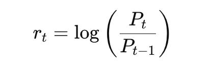
This transformation not only normalizes the data but also facilitates a more robust regression analysis by reducing heteroscedasticity. The regression model for predicting future returns can be formulated as:

Using historical log returns as predictors, we can forecast future return magnitudes and, by extension, price movements. Comparing predictions on return magnitudes versus the direction (i.e., sign) of returns often reveals that regression models may capture the intensity of movements even if the direction is less predictable.
Detailed Implementation Strategy for Algorithmic Trading
The strategy for predicting future returns via log returns is not merely an academic exercise; it’s a practical approach rooted in statistical properties beneficial for algorithmic trading. Here’s a more detailed breakdown:
Log Return Calculation: Stabilizing Time Series for Robust Analysis
Why Log Returns? In financial time series analysis, especially for algorithmic trading, stationarity is a crucial property. Stationary time series have statistical properties (like mean and variance) that do not change over time. Price levels themselves are often non-stationary, meaning their statistical properties vary, making them difficult to model directly. Log returns, defined as (image6.1), help transform price data into a more stationary series. This transformation is critical because most statistical and machine learning models, including linear regression, assume or perform better with stationary data.
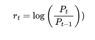
Heteroscedasticity Reduction: Another significant advantage of using log returns is the reduction of heteroscedasticity. Heteroscedasticity refers to the situation where the variance of the error term in a regression model is not constant. Financial time series, particularly price levels, often exhibit volatility clustering — periods of high volatility followed by periods of low volatility. Log transformation helps stabilize the variance, making regression models more reliable and efficient. This is vital for algorithmic trading systems that need consistent and predictable model performance across different market conditions.
Algorithmic Trading Perspective: For algorithmic trading systems, working with stationary series is paramount for building robust and backtestable strategies. Stationarity allows for the application of time-series models and techniques that rely on stable statistical properties. By calculating log returns, we’re essentially preprocessing the price data to make it more amenable to predictive modeling, which is the first step in building a predictive algorithmic trading strategy.
Lagged Return Features: Capturing Market Memory and Autocorrelation
Temporal Dependencies: Financial markets often exhibit autocorrelation, meaning that past returns can influence future returns, at least in the short term. This phenomenon is sometimes referred to as “market memory.” By constructing lagged values of log returns (i.e., image 6.2), we are creating features that capture these temporal dependencies. These lagged returns serve as predictors in our regression model, aiming to exploit the autocorrelative structure of financial returns.
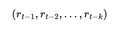
Supervised Dataset Construction: To train a regression model, we need a supervised dataset. By creating lagged features, we structure our data in a way that’s suitable for supervised learning. For each time (t), we use the lagged returns (image 6.3) as input features (independent variables) to predict the current return (r_t) (dependent variable). This step transforms the time series problem into a regression problem, which is a standard approach in predictive modeling.
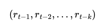
Algorithmic Trading Perspective: In algorithmic trading, identifying and exploiting patterns in market data is key. Autocorrelation in returns suggests that there might be predictable patterns that can be leveraged for trading. Using lagged returns as features is a direct way to model this autocorrelation. The number of lags ((k)) becomes a crucial parameter to tune, as it determines how far back into history the model looks to make predictions. This step is about feature engineering, a critical component in developing effective algorithmic trading strategies.
Regression Analysis: Vectorized Linear Regression for Efficiency
OLS Implementation: The strategy employs Ordinary Least Squares (OLS) regression to estimate the relationship between the lagged return features and the future return. OLS is a widely used and efficient method for linear regression, especially when implemented in a vectorized manner, which is crucial for handling large datasets in trading applications.
Parameter Estimation: The regression model (Image 6.4) aims to find the optimal values for the coefficients (Image 6.5). These coefficients quantify the relationship between each lagged return and the future return. The OLS method, especially via the normal equation, provides a direct way to compute these coefficients efficiently.
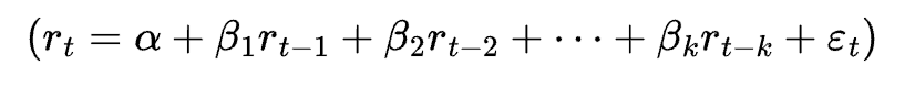
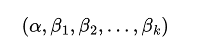
Vectorization for Speed: In algorithmic trading, speed and efficiency are essential. Vectorized operations in libraries like NumPy allow for fast computation of regression coefficients and predictions. This is in contrast to iterative or loop-based approaches, which can be significantly slower and less practical for real-time trading environments.
Algorithmic Trading Perspective: For algorithmic trading systems, the speed of model training and prediction is often critical. OLS regression, especially when vectorized, offers a computationally efficient method for return prediction. The estimated regression model becomes the core of the trading signal generation mechanism. The coefficients learned can be interpreted as a representation of market dynamics, according to the model assumptions.
Magnitude vs. Direction Comparison: Nuanced Model Evaluation for Trading Decisions
Magnitude Prediction: The regression model directly predicts the magnitude of future returns as a continuous value. This is valuable because in trading, the size of the expected return is as important as the direction. Knowing the magnitude helps in position sizing and risk management.
Direction Prediction: While the model predicts return magnitude, we can also derive directional predictions (up or down) by simply taking the sign of the predicted return. Comparing the performance of magnitude prediction versus direction prediction offers insights into what the model is actually capturing. It’s often found that predicting the magnitude of returns is statistically easier than predicting the direction with high accuracy.
Model Understanding and Refinement: Evaluating both magnitude and direction helps in understanding the strengths and limitations of the model. If the model is better at predicting magnitude than direction, it might be more effective for strategies that are less dependent on directional accuracy, or it might require further refinement to improve directional prediction.
Algorithmic Trading Perspective: In algorithmic trading, different strategies might prioritize either magnitude or direction prediction. For example, a volatility-based strategy might be more interested in predicting the magnitude of price movements, while a trend-following strategy might focus more on direction. By evaluating both aspects, we can better tailor the model and trading strategy to specific objectives. Moreover, understanding the model’s limitations is crucial for risk management and for making informed decisions about deploying the strategy in live trading.
Predicting Future Returns Using Log Returns
Let’s reimplement the code with a focus on modularity, clarity, and algorithmic trading context. We’ll break down the process into distinct functions for each key step, enhancing readability and reusability. We’ll also incorporate more sophisticated data handling and error checking.
import numpy as np
import pandas as pd

def calculate_log_returns(price_series: pd.Series) -> pd.Series:
    """
    Computes logarithmic returns from a price series.

    Args:
        price_series: Pandas Series of price levels.

    Returns:
        Pandas Series of log returns.
    """
    if not isinstance(price_series, pd.Series):
        raise ValueError("Input must be a Pandas Series.")
    if price_series.empty or len(price_series) < 2:
        return pd.Series([], dtype=float)  # Return empty series if insufficient data

    log_prices = np.log(price_series)
    log_returns = log_prices.diff().dropna() # Drop the first NaN resulting from diff
    return pd.Series(log_returns, index=price_series.index[1:]) # Align index


def create_lagged_features(return_series: pd.Series, num_lags: int) -> tuple[np.ndarray, np.ndarray]:
    """
    Constructs lagged features and target variable from a return series.

    Args:
        return_series: Pandas Series of returns.
        num_lags: Number of lagged returns to use as features.

    Returns:
        Tuple of feature matrix (X) and target vector (y).
    """
    if not isinstance(return_series, pd.Series):
        raise ValueError("Input must be a Pandas Series.")
    if return_series.empty or num_lags <= 0 or len(return_series) <= num_lags:
        return np.array([]), np.array([]) # Return empty arrays if insufficient data

    X_list, y_list = [], []
    for i in range(num_lags, len(return_series)):
        lags = return_series.iloc[i - num_lags:i].values
        target = return_series.iloc[i]
        X_list.append(lags)
        y_list.append(target)

    return np.array(X_list), np.array(y_list)


def ols_regression(X: np.ndarray, y: np.ndarray) -> np.ndarray:
    """
    Performs Ordinary Least Squares regression using the normal equation.

    Args:
        X: Feature matrix.
        y: Target vector.

    Returns:
        Numpy array of regression coefficients (beta).
    """
    if X.size == 0 or y.size == 0:
        return np.array([]) # Return empty array if no data

    try:
        XtX = X.T.dot(X)
        XtX_inv = np.linalg.inv(XtX)
        beta = XtX_inv.dot(X.T).dot(y)
        return beta
    except np.linalg.LinAlgError:
        raise ValueError("Singular matrix encountered in OLS regression. Check input data.")


def predict_next_return(X_last: np.ndarray, beta: np.ndarray) -> float:
    """
    Predicts the next return using the regression coefficients and the last set of lagged returns.

    Args:
        X_last: Array of the latest lagged return values.
        beta: Regression coefficients.

    Returns:
        Predicted next log return.
    """
    if X_last.size == 0 or beta.size == 0:
        return np.nan # Return NaN if input is invalid

    return X_last.dot(beta)


def evaluate_model_performance(predicted_returns: np.ndarray, actual_returns: np.ndarray) -> dict:
    """
    Evaluates the regression model's performance.

    Args:
        predicted_returns: Array of predicted returns.
        actual_returns: Array of actual returns.

    Returns:
        Dictionary of evaluation metrics (e.g., MSE, R-squared).
    """
    if predicted_returns.size == 0 or actual_returns.size == 0 or len(predicted_returns) != len(actual_returns):
        return {} # Return empty dict if no data or mismatched lengths

    mse = np.mean((predicted_returns - actual_returns) ** 2)
    # R-squared calculation
    ss_total = np.sum((actual_returns - np.mean(actual_returns)) ** 2)
    ss_residual = np.sum((actual_returns - predicted_returns) ** 2)
    r_squared = 1 - (ss_residual / ss_total) if ss_total > 0 else np.nan

    return {"Mean Squared Error": mse, "R-squared": r_squared}


def predict_future_returns_pipeline(prices: pd.Series, num_lags: int) -> float:
    """
    Pipeline function to predict future returns using lagged log returns and OLS.

    Args:
        prices: Pandas Series of historical price levels.
        num_lags: Number of lagged return values to use as features.

    Returns:
        Predicted future log return, or NaN if prediction is not possible.
    """
    if not isinstance(prices, pd.Series):
        raise ValueError("Input prices must be a Pandas Series.")
    if prices.empty or len(prices) <= num_lags + 1: # Need enough data for lags and prediction
        return np.nan # Not enough data to make prediction

    log_returns = calculate_log_returns(prices)
    if log_returns.empty or len(log_returns) <= num_lags:
        return np.nan # Not enough log returns after calculation

    X, y = create_lagged_features(log_returns, num_lags)
    if X.size == 0 or y.size == 0:
        return np.nan # No features could be created

    try:
        beta = ols_regression(X, y)
        if beta.size == 0:
            return np.nan # Regression failed to compute coefficients
        X_last = log_returns.tail(num_lags).values # Get the latest lagged returns as features
        predicted_log_return = predict_next_return(X_last, beta)
        return predicted_log_return
    except ValueError as e:
        print(f"Regression error: {e}") # Handle potential regression errors robustly
        return np.nan


# Example Usage (assuming you have historical price data in a Pandas Series called 'historical_prices')
if __name__ == '__main__':
    # Create a dummy price series for example
    dates = pd.date_range(start='2023-01-01', periods=200, freq='B') # Business days
    prices_data = np.cumsum(np.random.normal(0.0005, 0.01, 200)) + 100 # Simulate prices
    historical_prices = pd.Series(prices_data, index=dates)

    num_lags = 5  # Example number of lags
    predicted_return = predict_future_returns_pipeline(historical_prices, num_lags)

    if not np.isnan(predicted_return):
        print(f"Predicted Future Log Return: {predicted_return:.6f}")
        # Directional prediction (example)
        predicted_direction = "Up" if predicted_return > 0 else "Down" if predicted_return < 0 else "Neutral"
        print(f"Predicted Direction: {predicted_direction}")

        # Evaluate model (more meaningful evaluation would require out-of-sample testing)
        log_returns = calculate_log_returns(historical_prices)
        X, y = create_lagged_features(log_returns, num_lags)
        beta = ols_regression(X, y)
        if beta.size > 0: # Ensure beta coefficients were computed
            predicted_series = pd.Series([predict_next_return(x_row, beta) for x_row in X], index=log_returns.index[num_lags:])
            actual_series = log_returns.iloc[num_lags:]
            evaluation = evaluate_model_performance(predicted_series.values, actual_series.values)
            print("Model Evaluation:", evaluation)
    else:
        print("Could not generate a prediction due to insufficient data or errors.")
Detailed Explanation of the Code:
calculate_log_returns(price_series):
Takes a Pandas Series of prices as input.
Performs input validation to ensure it’s a Pandas Series and not empty.
Calculates log prices using
np.log().Computes the difference of log prices using
.diff()to get log returns.Handles the
NaNthat results from thediff()operation by dropping it using.dropna().Returns a Pandas Series of log returns, indexed to align correctly with the original price series (shifted by one period).
create_lagged_features(return_series, num_lags):
Accepts a Pandas Series of returns and the number of lags as input.
Validates the input Series and
num_lags.Iterates through the
return_seriesstarting from thenum_lags-th index. For each point, it extracts a window of lagged returns (of sizenum_lags) as features (X) and the current return as the target (y).Constructs feature matrix
Xand target vectoryas NumPy arrays.Returns the feature matrix and target vector.
ols_regression(X, y):
Takes the feature matrix
Xand target vectoryas input.Handles cases where input arrays are empty.
Implements the normal equation for OLS: (\beta = (X^T X)^{-1} X^T y).
Includes error handling for singular matrices (which can occur in multicollinearity or when (X^T X) is not invertible), raising a
ValueErrorif aLinAlgErroris encountered during matrix inversion.Returns the calculated regression coefficients
beta.
predict_next_return(X_last, beta):
Takes the last set of lagged returns
X_lastand the regression coefficientsbetaas input.Handles cases where input arrays are empty, returning
np.nanin such cases.Calculates the predicted next log return by performing a dot product of
X_lastandbeta:predicted_return = X_last · β.Returns the predicted log return as a float.
evaluate_model_performance(predicted_returns, actual_returns):
Takes arrays of predicted and actual returns to evaluate model performance.
Includes validation to ensure inputs are not empty and have matching lengths.
Calculates Mean Squared Error (MSE) as a measure of prediction accuracy.
Calculates R-squared to measure the proportion of variance in the dependent variable that is predictable from the independent variables. Handles the case where total sum of squares is zero to avoid division by zero.
Returns a dictionary containing evaluation metrics.
predict_future_returns_pipeline(prices, num_lags):
This function orchestrates the entire prediction pipeline.
It takes raw prices and
num_lagsas input.It performs a series of checks to ensure sufficient data at each step, returning
np.nanif data is insufficient or errors occur.It calls
calculate_log_returns,create_lagged_features,ols_regression, andpredict_next_returnin sequence to get the final prediction.Includes a try-except block to catch potential
ValueErrorfromols_regressionand handles it gracefully, returningnp.nan.Returns the predicted future log return or
np.nanif prediction is not possible.
Example Usage (if __name__ == '__main__':):
Provides a demonstration of how to use the
predict_future_returns_pipelinefunction.Creates a dummy price series for demonstration purposes.
Sets an example number of lags (
num_lags).Calls
predict_future_returns_pipelineto get a prediction.Prints the predicted return and derives a directional prediction (Up/Down/Neutral) from the sign of the predicted return.
Demonstrates a basic model evaluation using in-sample data, which is for illustration. For proper evaluation, out-of-sample or rolling window validation is necessary.
Predicting Market Direction
While forecasting the magnitude of returns is important, many trading strategies require a clear indication of market direction. Predicting the sign of the return transforms the regression problem into a classification problem. Here, rather than predicting a continuous return value, the goal is to predict whether the market will move upward or downward. A simple method is to assign a value of +1 if the predicted return is positive and -1 if negative:

This approach is particularly useful for trading strategies that rely on binary decisions. The hit ratio, or the percentage of times the predicted direction matches the actual market movement, becomes a critical performance metric. From a mathematical standpoint, by focusing on the sign rather than the magnitude, we can simplify the optimization problem and potentially improve the robustness of the trading signal, especially in highly volatile markets.
Implementation Strategy for Algorithmic Trading: Directional Prediction
Building on the foundation of return magnitude prediction, predicting market direction is a critical step towards actionable algorithmic trading strategies. Here’s a more in-depth look at each component of the strategy:
Regression on Log Returns: Leveraging Statistical Properties for Directional Clues
Directional Information Extraction: While the linear regression model, as previously described, primarily focuses on predicting the magnitude of future log returns, the sign of this prediction is inherently directional. A positive predicted log return suggests an upward price movement, and a negative one suggests a downward movement. This is the core concept for transforming a magnitude prediction into a directional forecast.
Assumptions and Limitations: It’s important to acknowledge that directly predicting market direction is inherently more challenging than predicting return magnitudes or volatility. Market direction is influenced by a multitude of factors, many of which are non-quantifiable or occur at very high frequencies (news events, sudden shifts in investor sentiment, etc.). Linear regression on lagged returns, while capturing some autocorrelation and statistical tendencies, is a simplification. It assumes that past return patterns have some predictive power for future direction, which may hold to varying degrees depending on market conditions and time horizons.
Market Efficiency Considerations: The efficiency of the market plays a crucial role here. In a perfectly efficient market, directional prediction based on historical prices alone would be theoretically impossible beyond pure chance. However, real-world markets exhibit varying degrees of inefficiency, especially in the short to medium term. This inefficiency can manifest as short-term autocorrelation or patterns that our regression model aims to exploit for directional predictions.
Algorithmic Trading Context: For algorithmic trading, even a slightly better than random directional prediction can be valuable, especially when combined with proper risk management and position sizing. The regression on log returns provides a statistically grounded method to generate these directional insights, which can then be translated into trading signals.
Sign Function Application and Thresholding: From Continuous Prediction to Discrete Signals
Basic Sign Function: The most straightforward approach is to apply a sign function directly to the predicted log return. If the predicted return (Image 6.6), we generate a buy signal (+1, indicating upward direction). If (image 6.7), we generate a sell signal (-1, downward direction). If (Image 6.8), we can either generate a neutral signal (0) or default to the previous position or no position.


Introducing Thresholds for Signal Refinement: A simple sign function might generate too many signals, some of which may be based on very small predicted returns and thus be noisy or unreliable. To refine the signal generation, we can introduce thresholds. For example:
Positive Threshold (Image 6.9): Only generate a buy signal (+1) if the predicted return (Image 6.10), where (Image 6.11 ).

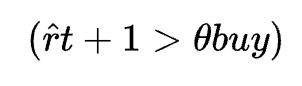

Negative Threshold (image 6.12): Only generate a sell signal (-1) if the predicted return ( Image 6.13 ), where ( Image 6.14).


Neutral Zone: If ( Image 6.15), we can consider the signal to be neutral (0), indicating no strong directional bias, or maintain the current position.
Threshold Optimization: The choice of thresholds ( \theta_{buy} ) and ( \theta_{sell} ) is crucial and can significantly impact the strategy’s performance. These thresholds can be optimized through backtesting and validation, potentially using techniques like grid search or more advanced optimization algorithms. The thresholds can be symmetric or asymmetric, depending on the market and strategy goals.
Algorithmic Trading Signal Generation: These threshold-based signals are directly actionable in an algorithmic trading system. A buy signal might trigger the system to enter a long position, a sell signal to enter a short position (or close a long position), and a neutral signal to do nothing. The thresholds control the sensitivity of the signal generation process and can be tuned to balance between signal frequency and signal quality.
Performance Evaluation: Beyond Hit Ratio — Comprehensive Metrics for Directional Strategies
Hit Ratio as a Basic Metric: The hit ratio (accuracy) — the percentage of times the predicted direction matches the actual market direction — is a primary metric for evaluating directional prediction. However, it’s important to recognize its limitations. A high hit ratio alone does not guarantee profitability, especially if winning trades are small and losing trades are large.
Profitability Metrics: For algorithmic trading, profitability is the ultimate goal. Therefore, performance evaluation must go beyond the hit ratio and include profitability metrics such as:
Total Return and Annualized Return: Measures the overall gain or loss over the backtesting period.
Risk-Adjusted Returns: Sharpe Ratio, Sortino Ratio, and Calmar Ratio, which account for the risk taken to achieve the returns (volatility, downside risk, maximum drawdown, respectively).
Profit Factor: Ratio of gross profit to gross loss, indicating the efficiency of the strategy in generating profit versus loss.
Maximum Drawdown: The largest peak-to-trough decline during the backtesting period, a critical measure of risk for many traders.
Statistical Significance and Robustness: It’s essential to assess the statistical significance of the results and the robustness of the strategy. This involves:
Statistical Tests: Performing statistical tests to check if the observed performance is statistically significantly better than random chance.
Out-of-Sample Testing: Evaluating the strategy on data not used for parameter optimization (out-of-sample or walk-forward testing) to assess generalization capability and avoid overfitting.
Sensitivity Analysis: Testing the strategy’s performance under different parameter settings (number of lags, thresholds, etc.) to understand its sensitivity to parameter choice.
Transaction Costs and Slippage: Incorporating realistic transaction costs (commissions, spread) and slippage in backtesting to get a more accurate picture of net profitability.
Algorithmic Trading Performance Assessment: A comprehensive performance evaluation is crucial for algorithmic trading strategy development. It not only tells us if the strategy is profitable on historical data but also provides insights into its risk profile, robustness, and potential for real-world deployment.
Integration with Backtesting Framework: From Prediction to Execution and Iteration
Seamless Signal Integration: The directional signals generated by our model (buy, sell, neutral) must be seamlessly integrated into a backtesting framework. This framework should be capable of simulating trades based on these signals, tracking portfolio positions, calculating returns, and applying transaction costs.
Iterative Strategy Development: Backtesting is not a one-time event; it’s an iterative process. The results of backtesting should inform further refinement of the prediction model and trading strategy. This might involve:
Parameter Tuning: Adjusting the number of lags, thresholds, regression parameters, etc., based on backtesting results.
Feature Engineering: Adding or modifying features used in the regression model.
Model Selection: Experimenting with different regression techniques or more complex machine learning models if linear regression proves insufficient.
Rule-Based Enhancements: Incorporating rule-based filters or conditions on top of the regression signals to improve signal quality or adapt to changing market conditions.
Algorithmic Trading System Lifecycle: Integration with a backtesting framework is a pivotal step in the lifecycle of an algorithmic trading system. It allows for rigorous testing, validation, and iterative improvement of the trading logic before deploying it in a live trading environment. It bridges the gap between theoretical prediction and practical execution.
Threshold-Based Directional Predictor
Let’s enhance the predict_market_direction function to incorporate thresholds for signal generation and maintain modularity by reusing the functions from the previous detailed code.
import numpy as np
import pandas as pd

# Assuming functions calculate_log_returns, create_lagged_features,
# ols_regression, predict_next_return, and predict_future_returns_pipeline
# are already defined as in the previous complex code example.
# We will reuse predict_future_returns_pipeline for predicting the log return.


def predict_market_direction_threshold(prices: pd.Series, num_lags: int, buy_threshold: float, sell_threshold: float) -> int:
    """
    Predict market direction using linear regression on lagged logarithmic returns with thresholds.
    The prediction is converted into a discrete signal: +1 for buy, -1 for sell, 0 for neutral.

    Args:
        prices: Pandas Series of historical price levels.
        num_lags: Number of lagged log return values to use as features.
        buy_threshold: Threshold above which a buy signal (+1) is generated.
        sell_threshold: Threshold below which a sell signal (-1) is generated.

    Returns:
        direction_signal: An integer, +1 for upward movement (buy), -1 for downward movement (sell), 0 for neutral.
    """
    if not isinstance(prices, pd.Series):
        raise ValueError("Input prices must be a Pandas Series.")
    if not isinstance(buy_threshold, (int, float)) or not isinstance(sell_threshold, (int, float)):
        raise TypeError("Thresholds must be numeric.")
    if buy_threshold <= sell_threshold:
        raise ValueError("Buy threshold must be greater than sell threshold.")


    predicted_log_return = predict_future_returns_pipeline(prices, num_lags)

    if np.isnan(predicted_log_return):
        return 0  # Return neutral signal if return prediction fails

    if predicted_log_return > buy_threshold:
        direction_signal = 1  # Buy signal
    elif predicted_log_return < sell_threshold:
        direction_signal = -1 # Sell signal
    else:
        direction_signal = 0  # Neutral signal

    return direction_signal


# Example Usage (assuming you have historical price data in a Pandas Series called 'historical_prices')
if __name__ == '__main__':
    # Create a dummy price series (same as before for consistency)
    dates = pd.date_range(start='2023-01-01', periods=200, freq='B') # Business days
    prices_data = np.cumsum(np.random.normal(0.0005, 0.01, 200)) + 100 # Simulate prices
    historical_prices = pd.Series(prices_data, index=dates)

    num_lags = 5         # Example number of lags
    buy_threshold = 0.001 # Example buy threshold (0.1%)
    sell_threshold = -0.001# Example sell threshold (-0.1%)

    direction_signal = predict_market_direction_threshold(historical_prices, num_lags, buy_threshold, sell_threshold)

    signal_interpretation = {1: "Buy", -1: "Sell", 0: "Neutral"}
    print(f"Predicted Market Direction Signal: {direction_signal} ({signal_interpretation[direction_signal]})")


    # --- Performance Evaluation (Illustrative - requires backtesting framework for proper assessment) ---
    # In a real algorithmic trading scenario, you would integrate this signal into a backtesting engine
    # and evaluate performance over a historical period, using metrics like Sharpe Ratio, Profit Factor, etc.
    # For a simple hit ratio calculation, you would need actual future returns to compare against the signals.
    # This part would be significantly more complex and depend on the backtesting framework.
    # For now, we just show how to get the signal.
predict_market_direction_threshold(prices, num_lags, buy_threshold, sell_threshold):