

Chapter 10 Algo Trading: Building a Financial Analysis Pipeline with Logistic Regression for Stock Predictions
A Comprehensive Approach to Data Processing, Feature Engineering, and Model Evaluation in Quantitative Finance

In this chapter, we'll delve into constructing a comprehensive financial analysis pipeline tailored for algorithmic trading. The goal is to build a predictive model using logistic regression, leveraging a variety of financial indicators—such as profitability, momentum, efficiency, and payout factors—to evaluate a stock's potential performance. This pipeline integrates essential steps like data cleaning, managing outliers, and transforming features to ensure robust model performance. With a time-series cross-validation approach, we can train the model on historical data and then test its predictive accuracy on future trends. This chapter provides a practical and scalable framework for incorporating logistic regression into quantitative finance analysis, enhancing your toolkit for algorithmic trading.
Read the previous chapters here:
jnkjnj
dfs
import pandas as pd
import numpy as np
from time import time
import talib
import re
from statsmodels.api import OLS
from sklearn.metrics import mean_squared_error
from scipy.stats import spearmanr
from sklearn.linear_model import LinearRegression, Ridge, RidgeCV, Lasso, LassoCV, LogisticRegression
from sklearn.preprocessing import StandardScaler

from quantopian.research import run_pipeline
from quantopian.pipeline import Pipeline, factors, filters, classifiers
from quantopian.pipeline.data.builtin import USEquityPricing
from quantopian.pipeline.factors import (Latest,
                                         Returns,
                                         AverageDollarVolume,
                                         SimpleMovingAverage,
                                         EWMA,
                                         BollingerBands,
                                         CustomFactor,
                                         MarketCap,
                                        SimpleBeta)
from quantopian.pipeline.filters import QTradableStocksUS, StaticAssets
from quantopian.pipeline.data.quandl import fred_usdontd156n as libor
from empyrical import max_drawdown, sortino_ratio

import seaborn as sns
import matplotlib.pyplot as plt
from sklearn.metrics import roc_auc_score
This code starts by bringing in several important libraries needed for handling data, performing statistical analysis, and building machine learning models. Let’s break down each part:
- Pandas and NumPy are loaded first. Pandas is excellent for working with data structures like tables (called DataFrames), while NumPy helps with numerical calculations.
- The time module is included to track how long certain operations take or to work with timestamps.
- talib is used for analyzing financial data. It offers various tools to calculate market indicators.
- The re library handles regular expressions, which are useful for cleaning or processing text data.
- statsmodels.api is imported for running Ordinary Least Squares (OLS) regression. This technique helps model relationships between different variables.
- From sklearn.metrics, two functions are brought in: mean_squared_error, which checks how well a regression model performs, and roc_auc_score, which evaluates classification models.
- Several regression models like LinearRegression, Ridge, and Lasso from sklearn.linear_model are included. This suggests that different methods will be tested to see which one works best.
- StandardScaler is also imported to standardize the data. This means adjusting the data so it has a mean of zero and a standard deviation of one, making it easier for models to process.
Next, the code imports tools related to Quantopian, which is a platform for quantitative research:
- The run_pipeline function, along with Pipeline, factors, filters, and classifiers, is used to set up and compute various factors on financial data.
- USEquityPricing gives access to stock pricing data, which is likely the main dataset being analyzed.
- Several financial indicators like Latest, Returns, and BollingerBands are set up. This means the code will calculate different market metrics for the stocks being studied.
Filters such as QTradableStocksUS ensure that only specific stocks, probably those that can be easily traded and meet certain criteria, are included in the analysis. Additionally, fred_usdontd156n brings in interest rate data, which might provide important context for the financial analysis.
Finally, the code imports plotting libraries seaborn and matplotlib.pyplot to create visualizations. Visualizing data and results is crucial for understanding and interpreting the models and findings.
In summary, this setup is designed to perform a comprehensive financial analysis. It involves organizing and cleaning data, running various statistical and machine learning models, and visualizing the results to understand financial trends and make predictions.
################
# Fundamentals #
################

# Morningstar fundamentals (2002 - Ongoing)
# https://www.quantopian.com/help/fundamentals
from quantopian.pipeline.data import Fundamentals

#####################
# Analyst Estimates #
#####################

# Earnings Surprises - Zacks (27 May 2006 - Ongoing)
# https://www.quantopian.com/data/zacks/earnings_surprises
from quantopian.pipeline.data.zacks import EarningsSurprises
from quantopian.pipeline.factors.zacks import BusinessDaysSinceEarningsSurprisesAnnouncement

##########
# Events #
##########

# Buyback Announcements - EventVestor (01 Jun 2007 - Ongoing)
# https://www.quantopian.com/data/eventvestor/buyback_auth
from quantopian.pipeline.data.eventvestor import BuybackAuthorizations
from quantopian.pipeline.factors.eventvestor import BusinessDaysSinceBuybackAuth

# CEO Changes - EventVestor (01 Jan 2007 - Ongoing)
# https://www.quantopian.com/data/eventvestor/ceo_change
from quantopian.pipeline.data.eventvestor import CEOChangeAnnouncements

# Dividends - EventVestor (01 Jan 2007 - Ongoing)
# https://www.quantopian.com/data/eventvestor/dividends
from quantopian.pipeline.data.eventvestor import (
    DividendsByExDate,
    DividendsByPayDate,
    DividendsByAnnouncementDate,
)
from quantopian.pipeline.factors.eventvestor import (
    BusinessDaysSincePreviousExDate,
    BusinessDaysUntilNextExDate,
    BusinessDaysSinceDividendAnnouncement,
)

# Earnings Calendar - EventVestor (01 Jan 2007 - Ongoing)
# https://www.quantopian.com/data/eventvestor/earnings_calendar
from quantopian.pipeline.data.eventvestor import EarningsCalendar
from quantopian.pipeline.factors.eventvestor import (
    BusinessDaysUntilNextEarnings,
    BusinessDaysSincePreviousEarnings
)

# 13D Filings - EventVestor (01 Jan 2007 - Ongoing)
# https://www.quantopian.com/data/eventvestor/_13d_filings
from quantopian.pipeline.data.eventvestor import _13DFilings
from quantopian.pipeline.factors.eventvestor import BusinessDaysSince13DFilingsDate

#############
# Sentiment #
#############

# News Sentiment - Sentdex Sentiment Analysis (15 Oct 2012 - Ongoing)
# https://www.quantopian.com/data/sentdex/sentiment
from quantopian.pipeline.data.sentdex import sentiment
This code sets up everything we need for a financial analysis project, focusing on using logistic regression to make predictions. Let’s break down each part to understand what’s happening.
Importing Essential Data
First, we bring in key data from Morningstar. This includes important figures like earnings, revenue, and other measures of a company’s financial health, going back to 2002. This information helps us see how a company has performed over time and serves as a foundation for our analysis.
Analyst Estimates and Earnings Surprises
Next, we use data from Zacks to look at analyst estimates, particularly earnings surprises. Earnings surprises occur when a company’s actual earnings differ from what analysts expected. These surprises can significantly affect stock prices. We also include a factor called BusinessDaysSinceEarningsSurprisesAnnouncement, which tracks how many business days have passed since the surprise was announced. This helps us analyze the impact over time.
Important Company Events
We then gather information from EventVestor about key company events. This includes buyback announcements, where a company plans to buy its own shares, which can be a positive sign for investors. We also track CEO changes, as new leadership can influence a company’s stock performance. Understanding these events helps us see how changes within a company might affect its stock.
Dividends Information
Dividends are another crucial part of our analysis because they show a company’s profitability and stability. We import various dividend-related data, such as the dates when dividends are declared (announcement dates), when they are paid out (pay dates), and the ex-dates, which determine who is eligible to receive the dividend. Additionally, we track how many business days have passed since these events or how many are left. This information helps us assess the company’s financial health and investor returns.
Earnings Calendar
The earnings calendar is also important. It provides a schedule of upcoming earnings announcements and notes how much time has passed since the last ones. This schedule helps us anticipate when new financial results will be released, which can influence stock prices based on the latest performance data.
Sentiment Analysis from News Articles
Finally, we include sentiment analysis from news articles. This means we analyze how news stories are talking about a company, whether the sentiment is positive, negative, or neutral. Understanding public perception and market sentiment helps us see how external opinions might influence a company’s stock performance.
Putting It All Together
All these data imports work together to create a strong foundation for our analysis. By combining financial indicators, company events, dividend information, earnings schedules, and market sentiment, we can use logistic regression to predict how these factors might impact stock performance. This comprehensive approach ensures that our predictions are based on a wide range of relevant information.
# trading days per period
MONTH = 21
YEAR = 12 * MONTH
This code sets up two important numbers that relate to trading days.
First, it defines MONTH as 21. This number represents the average number of trading days in a month, taking into account weekends and holidays when the markets are closed.
Then, it defines YEAR by multiplying 12 (the number of months in a year) by MONTH. This calculation gives us an annual total of 252 trading days (12 months × 21 trading days).
Using 252 trading days in a year is common in financial models because it focuses on the days when trading actually happens, rather than all the days on the calendar. This helps in making more accurate financial predictions and analyses.
START = '2014-01-01'
END = '2015-12-31'
In this step, you create two variables: START and END. These variables mark the beginning and end of the date range you want to analyze. Specifically, START is set to January 1, 2014, and END is set to December 31, 2015.
Choosing this timeframe is important because it allows you to filter your dataset to include only the records within these dates. By focusing on this specific period, you ensure that your logistic regression model is trained or tested using relevant data. Having clear start and end dates helps the model make more accurate predictions by using information that is most pertinent to your analysis.
def Q100US():
    return filters.make_us_equity_universe(
        target_size=100,
        rankby=factors.AverageDollarVolume(window_length=200),
        mask=filters.default_us_equity_universe_mask(),
        groupby=classifiers.fundamentals.Sector(),
        max_group_weight=0.3,
        smoothing_func=lambda f: f.downsample('month_start'),
    )
The Q100US function is designed to create a list of 100 U.S. stocks. It uses several steps to select and organize these stocks effectively.
First, the function sets a target size of 100, meaning it aims to include exactly 100 stocks in the final list. To choose these stocks, it ranks them based on their average dollar volume over the past 200 days. Average dollar volume measures how actively a stock has been traded, so this ranking helps pick the most actively traded stocks in the last 200 days.
Next, the function applies a default mask to the U.S. equity universe. Think of this mask as a filter that removes stocks that don’t meet certain criteria or aren’t suitable for the analysis. This step ensures that only qualified stocks are considered.
The selected stocks are then grouped by their sector using a sector classification system. This grouping helps create a diverse selection of stocks from different parts of the economy. To maintain this diversity, the function limits any single sector to a maximum of 30% of the total list. This cap prevents too many stocks from one sector, which could increase the overall risk of the portfolio.
Finally, the function uses a smoothing process to adjust the data to the beginning of each month. This downsampling makes the data more consistent and stable, which helps improve the accuracy of the stock rankings.
In summary, the Q100US function carefully filters and organizes U.S. stocks to create a balanced and actively traded list of 100 companies. This structured approach makes the stock selection process clear and manageable for further analysis or modeling.
# UNIVERSE = StaticAssets(symbols(['MSFT', 'AAPL']))
UNIVERSE = Q100US()
This piece of code sets up a variable named UNIVERSE, which determines the specific financial assets or stocks you want to analyze.
In the first line, which is commented out, there’s an option to define the universe by selecting particular stock symbols, such as Microsoft (MSFT) and Apple (AAPL). If you choose this option, your analysis will focus solely on these two companies.
However, the active line assigns UNIVERSE to Q100US(). This likely refers to a predefined group of the top 100 U.S. stocks based on certain factors like market size or how easily they can be bought and sold (known as liquidity). By using Q100US(), you include a wider variety of stocks in your analysis.
Using a broader set of stocks can improve your logistic regression analysis — a statistical method used to predict outcomes — by providing more data. This can lead to more accurate and reliable predictions.
class AnnualizedData(CustomFactor):
    # Get the sum of the last 4 reported values
    window_length = 260

    def compute(self, today, assets, out, asof_date, values):
        for asset in range(len(assets)):
            # unique asof dates indicate availability of new figures
            _, filing_dates = np.unique(asof_date[:, asset], return_index=True)
            quarterly_values = values[filing_dates[-4:], asset]
            # ignore annual windows with <4 quarterly data points
            if len(~np.isnan(quarterly_values)) != 4:
                out[asset] = np.nan
            else:
                out[asset] = np.sum(quarterly_values)
The AnnualizedData class is created to calculate the annualized figures for a group of assets using their most recent four quarterly values. Think of it as a specialized tool that fits into a bigger system for analyzing financial data.
The class uses a window_length of 260 days. This number is chosen because it covers enough trading days in a year to provide a reliable analysis.
When you run the compute method, it goes through each asset one by one. For each asset, it looks at the unique dates when new financial reports were filed, using the asof_date array. This step is crucial because it ensures we’re using the latest available data.
Next, the method pulls out the last four quarterly values for each asset based on these filing dates. It’s important to have exactly four quarterly values to calculate an accurate annual figure. If there are fewer than four values — perhaps because some data is missing — the method will return np.nan for that asset. This means there’s not enough information to compute a reliable annualized figure.
If there are four valid quarterly values, the method adds them up and saves this total in the output array for that asset. This annualized data can then be used in further analyses, such as running a logistic regression to make predictions based on these annual figures.
class AnnualAvg(CustomFactor):
    window_length = 252

    def compute(self, today, assets, out, values):
        out[:] = (values[0] + values[-1])/2
This code introduces a class named AnnualAvg, which is built on top of CustomFactor. In simple terms, CustomFactor is a tool used in financial software to perform specialized calculations, often within systems that test or execute trading strategies.
The window_length is set to 252. This number represents the typical number of trading days in a year, so setting the window length to 252 means we’re looking at data spanning one full year.
The main part of this class is the compute method. Here’s what it does:
1. Parameters Explained:
— today: The current date when the calculation is happening.
— assets: The financial assets (like stocks or bonds) that you’re analyzing.
— out: An array where the results of the calculation will be stored.
— values: A collection of data points covering the past 252 trading days.
2. Calculating the Annual Average:
— The method adds the first value in the values array to the last value.
— It then divides this sum by 2 to find the average of these two points.
— This average is saved into the out array for each asset being analyzed.
By using only the first and last values of the year, this method provides a simplified average. Instead of considering every single data point over the year, it focuses on just the starting and ending values. This makes the calculation faster and less complex, though it might overlook some variations that occur in between.
Overall, the AnnualAvg class offers a straightforward way to estimate yearly averages for financial assets, making it easier to integrate into larger trading or backtesting systems.
def factor_pipeline(factors):
    start = time()
    pipe = Pipeline({k: v(mask=UNIVERSE).rank() for k, v in factors.items()},
                    screen=UNIVERSE)
    result = run_pipeline(pipe, start_date=START, end_date=END)
    return result, time() - start
The factor_pipeline function is built to handle financial factors used for making predictions, typically within a trading strategy.
First, it records the current time to track how long the process takes. Then, it creates a Pipeline object. This pipeline uses a dictionary comprehension, which loops through each item in the factors dictionary. For every factor, it applies a mask using a predefined UNIVERSE. Think of the UNIVERSE as the set of all stocks or assets you’re considering. The mask filters the data to include only those within this universe. After filtering, it ranks the data using the rank() method. Ranking helps prioritize the most important factors within your investment universe.
Once the pipeline is set up, the function runs it using the run_pipeline() function. This function takes the created pipeline and a specific date range, defined by START and END. The output from running the pipeline, which includes the processed factor data, is stored in the result variable.
Finally, the function returns two things: the result of the pipeline execution and the time it took to run the entire process. The time is calculated by subtracting the start time from the current time. Keeping track of how long the process takes is useful for monitoring performance, especially when you’re testing different factors or running multiple pipelines at the same time.
class ValueFactors:
    """Definitions of factors for cross-sectional trading algorithms"""

    @staticmethod
    def PriceToSalesTTM(**kwargs):
        """Last closing price divided by sales per share"""
        return Fundamentals.ps_ratio.latest

    @staticmethod
    def PriceToEarningsTTM(**kwargs):
        """Closing price divided by earnings per share (EPS)"""
        return Fundamentals.pe_ratio.latest

    @staticmethod
    def PriceToDilutedEarningsTTM(mask):
        """Closing price divided by diluted EPS"""
        last_close = USEquityPricing.close.latest
        diluted_eps = AnnualizedData(inputs = [Fundamentals.diluted_eps_earnings_reports_asof_date,
                                               Fundamentals.diluted_eps_earnings_reports],
                                     mask=mask)
        return last_close / diluted_eps

    @staticmethod
    def PriceToForwardEarnings(**kwargs):
        """Price to Forward Earnings"""
        return Fundamentals.forward_pe_ratio.latest

    @staticmethod
    def DividendYield(**kwargs):
        """Dividends per share divided by closing price"""
        return Fundamentals.trailing_dividend_yield.latest

    @staticmethod
    def PriceToFCF(mask):
        """Price to Free Cash Flow"""
        last_close = USEquityPricing.close.latest
        fcf_share = AnnualizedData(inputs = [Fundamentals.fcf_per_share_asof_date,
                                             Fundamentals.fcf_per_share],
                                   mask=mask)
        return last_close / fcf_share

    @staticmethod
    def PriceToOperatingCashflow(mask):
        """Last Close divided by Operating Cash Flows"""
        last_close = USEquityPricing.close.latest
        cfo_per_share = AnnualizedData(inputs = [Fundamentals.cfo_per_share_asof_date,
                                                 Fundamentals.cfo_per_share],
                                       mask=mask)
        return last_close / cfo_per_share

    @staticmethod
    def PriceToBook(mask):
        """Closing price divided by book value"""
        last_close = USEquityPricing.close.latest
        book_value_per_share = AnnualizedData(inputs = [Fundamentals.book_value_per_share_asof_date,
                                              Fundamentals.book_value_per_share],
                                             mask=mask)
        return last_close / book_value_per_share


    @staticmethod
    def EVToFCF(mask):
        """Enterprise Value divided by Free Cash Flows"""
        fcf = AnnualizedData(inputs = [Fundamentals.free_cash_flow_asof_date,
                                       Fundamentals.free_cash_flow],
                             mask=mask)
        return Fundamentals.enterprise_value.latest / fcf

    @staticmethod
    def EVToEBITDA(mask):
        """Enterprise Value to Earnings Before Interest, Taxes, Deprecation and Amortization (EBITDA)"""
        ebitda = AnnualizedData(inputs = [Fundamentals.ebitda_asof_date,
                                          Fundamentals.ebitda],
                                mask=mask)

        return Fundamentals.enterprise_value.latest / ebitda

    @staticmethod
    def EBITDAYield(mask):
        """EBITDA divided by latest close"""
        ebitda = AnnualizedData(inputs = [Fundamentals.ebitda_asof_date,
                                          Fundamentals.ebitda],
                                mask=mask)
        return USEquityPricing.close.latest / ebitda
This code defines a class called ValueFactors that includes several methods for calculating financial ratios. These ratios are essential for cross-sectional trading algorithms, which analyze and compare different stocks. Each method in the class uses data from a source named Fundamentals and the latest closing prices from USEquityPricing to compute specific financial metrics.
Here are some of the main methods and what they do:
- PriceToSalesTTM: This calculates the price-to-sales ratio by dividing the latest closing price of a stock by its most recent sales per share. It helps investors understand how much they’re paying for each dollar of the company’s sales.
- PriceToEarningsTTM: This method computes the price-to-earnings (P/E) ratio. The P/E ratio shows how much investors are willing to pay for each dollar of the company’s earnings, providing insight into the stock’s valuation.
- PriceToDilutedEarningsTTM: Similar to the P/E ratio, this divides the latest closing price by diluted earnings per share. It’s especially useful when considering potential increases in shares due to stock options or convertible securities.
- PriceToForwardEarnings: This ratio is like the P/E ratio but uses future earnings estimates. It helps assess the company’s expected profitability based on projected earnings.
- DividendYield: This calculates the dividend yield by dividing dividends per share by the closing price. It measures the return investors receive from dividends relative to the stock price.
- PriceToFCF: This ratio divides the stock price by free cash flow (FCF). It indicates how much investors are paying for each dollar of the company’s free cash flow, which is important for understanding the company’s cash generation.
- PriceToOperatingCashflow: Here, the latest closing price is divided by the operating cash flows. This ratio provides insight into how the stock price relates to the company’s operational efficiency.
- PriceToBook: This ratio compares the closing price to the book value of the company. It helps investors understand how the market values the company’s assets.
- EVToFCF and EVToEBITDA: These methods calculate ratios using the enterprise value (EV) of the company. EVToFCF divides EV by free cash flow, and EVToEBITDA divides EV by earnings before interest, taxes, depreciation, and amortization (EBITDA). These ratios help assess the company’s overall valuation in relation to its earnings and cash generation.
- EBITDAYield: This calculates the EBITDA yield by dividing EBITDA by the latest closing price. It measures the company’s operational profitability compared to its market price.
Most of these methods use a mask parameter, which acts as a filter to select specific data points during the calculations. This allows the methods to focus on relevant data when computing the ratios. Additionally, the AnnualizedData class is used alongside the financial fundamentals to manage dates and filters effectively, ensuring that only pertinent data is processed.
Each method returns a numerical value representing the calculated ratio. These values can then be used for further analysis or incorporated into trading strategies to make informed investment decisions.
VALUE_FACTORS = {
    'DividendYield'            : ValueFactors.DividendYield,
    'EBITDAYield'              : ValueFactors.EBITDAYield,
    'EVToEBITDA'               : ValueFactors.EVToEBITDA,
    'EVToFCF'                  : ValueFactors.EVToFCF,
    'PriceToBook'              : ValueFactors.PriceToBook,
    'PriceToDilutedEarningsTTM': ValueFactors.PriceToDilutedEarningsTTM,
    'PriceToEarningsTTM'       : ValueFactors.PriceToEarningsTTM,
    'PriceToFCF'               : ValueFactors.PriceToFCF,
    'PriceToForwardEarnings'   : ValueFactors.PriceToForwardEarnings,
    'PriceToOperatingCashflow' : ValueFactors.PriceToOperatingCashflow,
    'PriceToSalesTTM'          : ValueFactors.PriceToSalesTTM,
}
This code defines a dictionary called VALUE_FACTORS. A dictionary is a way to store data using pairs of keys and values. In this case, the keys are descriptive names like ‘DividendYield’ and ‘PriceToEarningsTTM’. Each key is linked to a specific attribute from the ValueFactors class or module.
Each key in the dictionary represents a financial metric that is useful for evaluating or analyzing a company. The values associated with these keys are references to methods or calculations within the ValueFactors structure. These methods take care of retrieving or computing the necessary data for each metric.
For example, if you want to get the earnings metric, you can use the key ‘PriceToEarningsTTM’. When you use this key, the code accesses the corresponding method in ValueFactors to get the earnings information.
Using this dictionary makes the code simpler and easier to manage. All the value factors are organized in one place, so you can quickly find and use them by their names. This approach improves the readability of the code and makes it easier to update or maintain in the future.
value_result, t = factor_pipeline(VALUE_FACTORS)
print('Pipeline run time {:.2f} secs'.format(t))
value_result.info()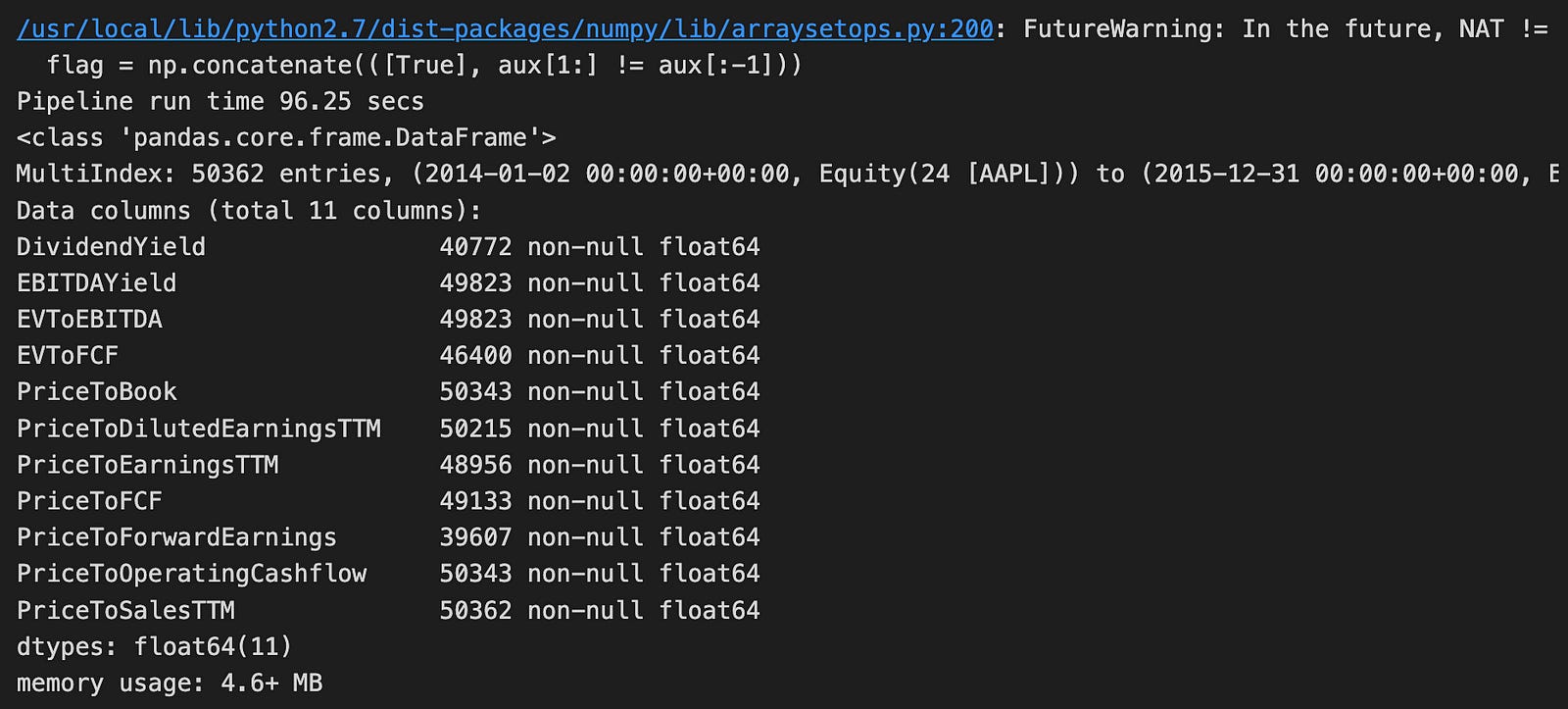
The code runs a function named factor_pipeline using VALUE_FACTORS as input. This function probably handles financial data related to stock factors. When it finishes, it returns two things: value_result, which holds the processed data, and t, which records how long the pipeline took to run. The print statement shows that the pipeline completed in about 96.25 seconds.
Looking at the output, we see that the data is in a Pandas DataFrame with 50,362 rows and 11 columns. This is a large dataset, likely containing historical financial information for a specific stock, such as Apple Inc. (AAPL). Each column includes different financial metrics like Dividend Yield, EBITDA Yield, and various price ratios. These metrics are important for assessing a company’s financial health and making investment decisions. Additionally, each column has no missing values, which is important for accurate analysis.
The DataFrame uses 4.6 MB of memory, which is quite efficient given its size. There is a warning about future changes in how NaT (Not a Time) values are handled. This means the code might need updates in future library versions, but it doesn’t impact the current run. Overall, this code snippet and its output show how financial data is prepared for further analysis, potentially to predict stock performance using logistic regression.
class MomentumFactors:
    """Custom Momentum Factors"""
    class PercentAboveLow(CustomFactor):
        """Percentage of current close above low
        in lookback window of window_length days
        """
        inputs = [USEquityPricing.close]
        window_length = 252

        def compute(self, today, assets, out, close):
            out[:] = close[-1] / np.min(close, axis=0) - 1

    class PercentBelowHigh(CustomFactor):
        """Percentage of current close below high
        in lookback window of window_length days
        """

        inputs = [USEquityPricing.close]
        window_length = 252

        def compute(self, today, assets, out, close):
            out[:] = close[-1] / np.max(close, axis=0) - 1

    @staticmethod
    def make_dx(timeperiod=14):
        class DX(CustomFactor):
            """Directional Movement Index"""
            inputs = [USEquityPricing.high,
                      USEquityPricing.low,
                      USEquityPricing.close]
            window_length = timeperiod + 1

            def compute(self, today, assets, out, high, low, close):
                out[:] = [talib.DX(high[:, i],
                                   low[:, i],
                                   close[:, i],
                                   timeperiod=timeperiod)[-1]
                          for i in range(len(assets))]
        return DX

    @staticmethod
    def make_mfi(timeperiod=14):
        class MFI(CustomFactor):
            """Money Flow Index"""
            inputs = [USEquityPricing.high,
                      USEquityPricing.low,
                      USEquityPricing.close,
                      USEquityPricing.volume]
            window_length = timeperiod + 1

            def compute(self, today, assets, out, high, low, close, vol):
                out[:] = [talib.MFI(high[:, i],
                                    low[:, i],
                                    close[:, i],
                                    vol[:, i],
                                    timeperiod=timeperiod)[-1]
                          for i in range(len(assets))]
        return MFI

    @staticmethod
    def make_oscillator(fastperiod=12, slowperiod=26, matype=0):
        class PPO(CustomFactor):
            """12/26-Day Percent Price Oscillator"""
            inputs = [USEquityPricing.close]
            window_length = slowperiod

            def compute(self, today, assets, out, close_prices):
                out[:] = [talib.PPO(close,
                                    fastperiod=fastperiod,
                                    slowperiod=slowperiod,
                                    matype=matype)[-1]
                         for close in close_prices.T]
        return PPO

    @staticmethod
    def make_stochastic_oscillator(fastk_period=5, slowk_period=3, slowd_period=3,
                                   slowk_matype=0, slowd_matype=0):
        class StochasticOscillator(CustomFactor):
            """20-day Stochastic Oscillator """
            inputs = [USEquityPricing.high,
                      USEquityPricing.low,
                      USEquityPricing.close]
            outputs = ['slowk', 'slowd']
            window_length = fastk_period * 2

            def compute(self, today, assets, out, high, low, close):
                slowk, slowd = [talib.STOCH(high[:, i],
                                            low[:, i],
                                            close[:, i],
                                            fastk_period=fastk_period,
                                            slowk_period=slowk_period,
                                            slowk_matype=slowk_matype,
                                            slowd_period=slowd_period,
                                            slowd_matype=slowd_matype)[-1]
                                for i in range(len(assets))]

                out.slowk[:], out.slowd[:] = slowk[-1], slowd[-1]
        return StochasticOscillator

    @staticmethod
    def make_trendline(timeperiod=252):
        class Trendline(CustomFactor):
            inputs = [USEquityPricing.close]
            """52-Week Trendline"""
            window_length = timeperiod

            def compute(self, today, assets, out, close_prices):
                out[:] = [talib.LINEARREG_SLOPE(close,
                                   timeperiod=timeperiod)[-1]
                          for close in close_prices.T]
        return Trendline
This code introduces a class called MomentumFactors, which bundles several custom financial indicators based on stock price data. Each indicator is defined as its own inner class within MomentumFactors, allowing them to handle their specific calculations and inputs independently. Let’s walk through each part:
1. PercentAboveLow: This indicator measures how much the current closing price of a stock is above its lowest price over the past 252 days (roughly one trading year). It calculates this by dividing today’s closing price by the lowest closing price in that period and then subtracting 1 to get a percentage.
2. PercentBelowHigh: Similar to PercentAboveLow, this indicator shows how much the current closing price is below the highest price in the last 252 days. It uses the same method of division to express the difference as a percentage.
3. make_dx: This method creates a class for the Directional Movement Index (DMI), a tool that helps identify the direction of a stock’s trend. You can set the number of days it looks back, with the default being 14 days. The compute function within this class uses the TA-Lib DX function to calculate the DMI for each stock.
4. make_mfi: This method sets up a class for the Money Flow Index (MFI), which tracks the flow of money into and out of a stock. Like the DMI, it typically looks back 14 days and uses both price and volume data. The TA-Lib MFI function performs the actual calculation.
5. make_oscillator: This static method creates a Percent Price Oscillator (PPO) class. The PPO compares two moving averages of a stock’s closing prices — a faster one (default 12 days) and a slower one (default 26 days). It uses the TA-Lib PPO function to determine the oscillator’s value.
6. make_stochastic_oscillator: This method builds a Stochastic Oscillator class, which calculates both fast and slow stochastic values to assess a stock’s momentum. It uses various settings like time periods and types of moving averages, relying on TA-Lib functions to perform the calculations.
7. make_trendline: This static method creates a trendline class that calculates the slope of a line fitted to the closing prices over a set period (default is 252 days). It uses the LINEARREG_SLOPE function from TA-Lib to determine the slope, indicating the trend’s direction and strength.
In summary, the MomentumFactors class and its inner classes provide a structured way to calculate different technical indicators used in momentum trading strategies. They leverage the TA-Lib library for mathematical calculations, making each indicator easy to use, modify, and expand upon as needed.
MOMENTUM_FACTORS = {
    'Percent Above Low'            : MomentumFactors.PercentAboveLow,
    'Percent Below High'           : MomentumFactors.PercentBelowHigh,
    'Price Oscillator'             : MomentumFactors.make_oscillator(),
    'Money Flow Index'             : MomentumFactors.make_mfi(),
    'Directional Movement Index'   : MomentumFactors.make_dx(),
    'Trendline'                    : MomentumFactors.make_trendline()
}
This code snippet sets up a dictionary named MOMENTUM_FACTORS. This dictionary links easy-to-understand names to specific methods or properties from the MomentumFactors class. Each pair in the dictionary represents a different momentum indicator you can use to analyze financial data.
- Descriptive Keys: Names like ‘Percent Above Low’ and ‘Percent Below High’ clearly describe what they measure. For example, ‘Percent Above Low’ likely indicates how much the current price is above the lowest price over a certain time period, while ‘Percent Below High’ shows how much it’s below the highest price. These keys are connected to corresponding attributes in the MomentumFactors class, such as MomentumFactors.PercentAboveLow.
- Method-Based Entries: Some entries use methods to calculate their values. Indicators like the Price Oscillator, Money Flow Index, and Directional Movement Index are computed using functions like MomentumFactors.make_oscillator(), MomentumFactors.make_mfi(), and MomentumFactors.make_dx(). These methods probably return the calculated values or objects for each momentum indicator.
- Trendline Calculation: The entry MomentumFactors.make_trendline() suggests there’s a special method for calculating trendlines based on price data.
By using the MOMENTUM_FACTORS dictionary, you can easily access and manage these different momentum indicators by their names. This organized approach makes it simpler to incorporate multiple indicators into your financial analysis or modeling tasks without getting bogged down by complex code.
momentum_result, t = factor_pipeline(MOMENTUM_FACTORS)
print('Pipeline run time {:.2f} secs'.format(t))
momentum_result.info()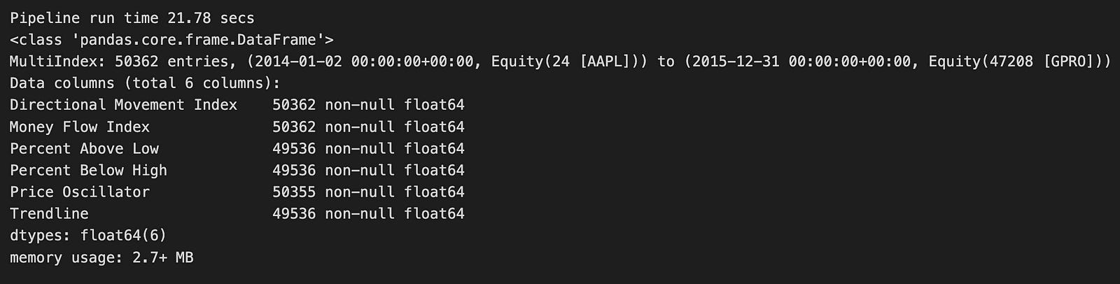
The code runs a function named factor_pipeline using MOMENTUM_FACTORS as its input. These momentum factors are financial indicators that help evaluate the strength and direction of stock price movements. When the function executes, it returns two things: momentum_result, which holds the processed data, and t, which shows how long the pipeline took to run. A print statement then displays the runtime, showing that the pipeline finished in about 21.78 seconds.
Looking at the output, momentum_result is a Pandas DataFrame. If you’re not familiar, a DataFrame is a table-like structure in Python that’s great for organizing and analyzing data. This particular DataFrame has 50,362 rows, indicating a large dataset. It likely covers multiple time periods for Apple Inc. (AAPL), with data ranging from January 2, 2014, to December 31, 2015. This timeframe gives a clear window for examining Apple’s stock performance.
The DataFrame includes six columns, each representing a different momentum indicator:
1. Directional Movement Index: Measures the strength of a price trend.
2. Money Flow Index: Assesses buying and selling pressure.
3. Percent Above Low: Shows how much the current price is above the low price.
4. Percent Below High: Indicates how much the current price is below the high price.
5. Price Oscillator: Highlights the difference between two moving averages.
6. Trendline: Identifies the general direction of the stock price.
Most of these columns have a high number of non-null entries, meaning the data is largely complete and reliable for analysis. The DataFrame uses about 2.7 MB of memory, which is efficient given the size of the dataset.
In summary, this code snippet runs a financial analysis focused on momentum factors. It produces a well-organized dataset that can be used for further analysis, such as building models to predict stock price movements based on past trends.
class EfficiencyFactors:

    @staticmethod
    def CapexToAssets(mask):
        """Capital Expenditure divided by Total Assets"""
        capex = AnnualizedData(inputs = [Fundamentals.capital_expenditure_asof_date,
                                         Fundamentals.capital_expenditure],
                                     mask=mask)
        assets = Fundamentals.total_assets.latest
        return - capex / assets

    @staticmethod
    def CapexToSales(mask):
        """Capital Expenditure divided by Total Revenue"""
        capex = AnnualizedData(inputs = [Fundamentals.capital_expenditure_asof_date,
                                         Fundamentals.capital_expenditure],
                                     mask=mask)
        revenue = AnnualizedData(inputs = [Fundamentals.total_revenue_asof_date,
                                         Fundamentals.total_revenue],
                                     mask=mask)
        return - capex / revenue

    @staticmethod
    def CapexToFCF(mask):
        """Capital Expenditure divided by Free Cash Flows"""
        capex = AnnualizedData(inputs = [Fundamentals.capital_expenditure_asof_date,
                                         Fundamentals.capital_expenditure],
                                     mask=mask)
        free_cash_flow = AnnualizedData(inputs = [Fundamentals.free_cash_flow_asof_date,
                                         Fundamentals.free_cash_flow],
                                     mask=mask)
        return - capex / free_cash_flow

    @staticmethod
    def EBITToAssets(mask):
        """Earnings Before Interest and Taxes (EBIT) divided by Total Assets"""
        ebit = AnnualizedData(inputs = [Fundamentals.ebit_asof_date,
                                         Fundamentals.ebit],
                                     mask=mask)
        assets = Fundamentals.total_assets.latest
        return ebit / assets

    @staticmethod
    def CFOToAssets(mask):
        """Operating Cash Flows divided by Total Assets"""
        cfo = AnnualizedData(inputs = [Fundamentals.operating_cash_flow_asof_date,
                                         Fundamentals.operating_cash_flow],
                                     mask=mask)
        assets = Fundamentals.total_assets.latest
        return cfo / assets

    @staticmethod
    def RetainedEarningsToAssets(mask):
        """Retained Earnings divided by Total Assets"""
        retained_earnings = AnnualizedData(inputs = [Fundamentals.retained_earnings_asof_date,
                                         Fundamentals.retained_earnings],
                                     mask=mask)
        assets = Fundamentals.total_assets.latest
        return retained_earnings / assets
The code defines a class named EfficiencyFactors that includes several static methods for calculating important financial ratios. These ratios help assess a company’s operational efficiency and overall financial health.
Each method uses a parameter called mask, which likely filters or specifies the data needed for the calculation. The class computes six key ratios:
1. Capex to Assets: This method calculates the ratio of Capital Expenditure (Capex) to Total Assets. It obtains Capex data using the AnnualizedData class, which collects data based on certain inputs and applies the provided mask. Total Assets are retrieved directly from the Fundamentals class. The ratio is returned as the negative value of Capex divided by Assets.
2. Capex to Sales: This method determines the ratio of Capex to Total Revenue. Like the first method, it gathers Capex data and also retrieves Revenue data using AnnualizedData. The result is the negative ratio of Capex to Revenue.
3. Capex to Free Cash Flows (FCF): Here, the ratio of Capex to Free Cash Flows is calculated. Capex and Free Cash Flow data are both obtained using AnnualizedData. The method returns the negative ratio of Capex to FCF.
4. EBIT to Assets: This method computes the ratio of Earnings Before Interest and Taxes (EBIT) to Total Assets. EBIT data is sourced through AnnualizedData, while Total Assets come from the Fundamentals class. Unlike the Capex ratios, this ratio is positive, showing how effectively the company’s assets generate earnings.
5. CFO to Assets: This method evaluates the ratio of Operating Cash Flows (CFO) to Total Assets. It retrieves CFO data and Total Assets, providing insight into how efficiently the company’s assets generate cash.
6. Retained Earnings to Assets: This method calculates the ratio of Retained Earnings to Total Assets. Retained Earnings data is fetched using AnnualizedData, similar to the other methods, and then divided by Total Assets.
Overall, these methods offer a simple way to analyze different aspects of a company’s financial performance using standard ratios. Since the methods are static, you can use them directly through the EfficiencyFactors class without creating an instance of it. This makes it easy to access and use these calculations for financial analysis.
EFFICIENCY_FACTORS = {
    'CFO To Assets' :EfficiencyFactors.CFOToAssets,
    'Capex To Assets' :EfficiencyFactors.CapexToAssets,
    'Capex To FCF' :EfficiencyFactors.CapexToFCF,
    'Capex To Sales' :EfficiencyFactors.CapexToSales,
    'EBIT To Assets' :EfficiencyFactors.EBITToAssets,
    'Retained Earnings To Assets' :EfficiencyFactors.RetainedEarningsToAssets
    }
This piece of code creates a dictionary called EFFICIENCY_FACTORS. In this dictionary, each key is a string that names a specific financial metric, and each value comes from the EfficiencyFactors class or module.
For example, the key ‘CFO To Assets’ is linked to EfficiencyFactors.CFOToAssets, which probably contains a number or a function related to that metric. Think of the dictionary as an organized collection of these efficiency metrics. This setup makes it easy to reference each metric by its name.
Using EFFICIENCY_FACTORS improves the readability of your code and allows you to quickly find and use these values later on. Whether you’re analyzing data or building a model, having these metrics organized in a clear way helps streamline your work.
efficiency_result, t = factor_pipeline(EFFICIENCY_FACTORS)
print('Pipeline run time {:.2f} secs'.format(t))
efficiency_result.info()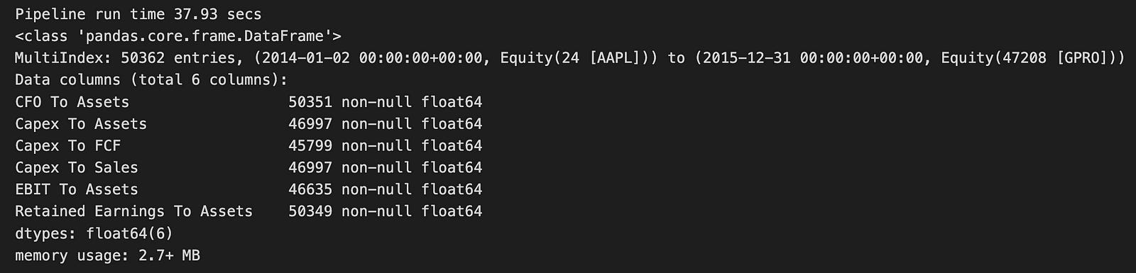
The code runs a function named factor_pipeline, which analyzes a set of efficiency factors — likely financial metrics related to companies. This function returns two things: efficiency_result, a DataFrame that holds the processed data, and t, which is the time it took to execute the pipeline in seconds. When printed, it shows that the pipeline finished in about 37.93 seconds.
Looking at the output, efficiency_result is a pandas DataFrame with a multi-index, meaning the data is organized by both date and equity identifiers. It includes 50,362 entries covering the period from January 2, 2014, to December 31, 2015, and encompasses various equity assets. The DataFrame has six columns, each representing different financial ratios or metrics:
1. CFO to Assets: Cash Flow from Operations relative to Assets
2. Capex to Assets: Capital Expenditures relative to Assets
3. Capex to FCF: Capital Expenditures relative to Free Cash Flow
4. Capex to Sales: Capital Expenditures relative to Sales
5. EBIT to Assets: Earnings Before Interest and Taxes relative to Assets
6. Retained Earnings to Assets: Retained Earnings relative to Assets
All these columns contain numerical values in the float64 format, and there are no missing entries, ensuring the dataset is complete for the specified metrics.
The DataFrame uses a bit over 2.7 MB of memory, which is quite efficient given the volume of data. This output offers a clear snapshot of the financial efficiency metrics for the selected equities, making it suitable for further analysis or modeling, such as using logistic regression for predictions. The well-structured format of the DataFrame makes it easy to manipulate and explore the data, which is crucial for gaining insights in financial analysis.
class RiskFactors:

    @staticmethod
    def LogMarketCap(mask):
        """Log of Market Capitalization log(Close Price * Shares Outstanding)"""
        return np.log(MarketCap(mask=mask))

    class DownsideRisk(CustomFactor):
        """Mean returns divided by std of 1yr daily losses (Sortino Ratio)"""
        inputs = [USEquityPricing.close]
        window_length = 252

        def compute(self, today, assets, out, close):
            ret = pd.DataFrame(close).pct_change()
            out[:] = ret.mean().div(ret.where(ret<0).std())

    @staticmethod
    def MarketBeta(**kwargs):
        """Slope of 1-yr regression of price returns against index returns"""
        return SimpleBeta(target=symbols('SPY'), regression_length=252)

    class DownsideBeta(CustomFactor):
        """Slope of 1yr regression of returns on negative index returns"""
        inputs = [USEquityPricing.close]
        window_length = 252

        def compute(self, today, assets, out, close):
            t = len(close)
            assets = pd.DataFrame(close).pct_change()

            start_date = (today - pd.DateOffset(years=1)).strftime('%Y-%m-%d')
            spy = get_pricing('SPY',
                              start_date=start_date,
                              end_date=today.strftime('%Y-%m-%d')).reset_index(drop=True)
            spy_neg_ret = (spy
                           .close_price
                           .iloc[-t:]
                           .pct_change()
                           .pipe(lambda x: x.where(x<0)))

            out[:] = assets.apply(lambda x: x.cov(spy_neg_ret)).div(spy_neg_ret.var())

    class Vol3M(CustomFactor):
        """3-month Volatility: Standard deviation of returns over 3 months"""

        inputs = [USEquityPricing.close]
        window_length = 63

        def compute(self, today, assets, out, close):
            out[:] = np.log1p(pd.DataFrame(close).pct_change()).std()
The RiskFactors class is a collection of tools designed to analyze financial risk. It includes various methods and nested classes that perform common financial calculations, making it easier to assess and manage investment risks.
LogMarketCap Method
The LogMarketCap method calculates the logarithm of a company’s market capitalization. To do this, it multiplies the stock’s closing price by the number of shares outstanding and then takes the natural logarithm of that total. This transformation helps to smooth out extreme values in market cap data, making it simpler to analyze and compare different companies.
DownsideRisk Class
Next, we have the DownsideRisk class, which extends a custom factor for financial analysis. This class calculates the Sortino Ratio, a measure of an asset’s risk-adjusted return. Here’s how it works:
1. It looks at the stock’s returns over the past year, which typically includes 252 trading days.
2. It calculates the daily percentage changes in the closing prices to determine the returns.
3. It finds the average of these returns.
4. It then divides this average by the standard deviation of only the negative returns (losses).
The Sortino Ratio focuses specifically on downside risk, giving investors a clearer picture of how well an asset performs relative to the risks of losing money.
MarketBeta Method
The MarketBeta method measures a stock’s volatility compared to the overall market, represented by the SPY index. Beta is a key indicator of how much a stock’s price moves in relation to the market:
1. It performs a regression analysis, which is a statistical method, over the past year.
2. The result tells you how much the stock tends to move when the market goes up or down.
A higher beta means the stock is more volatile, while a lower beta indicates it is more stable.
DownsideBeta Class
The DownsideBeta class is another custom factor that looks at how a stock reacts during market downturns. Here’s what it does:
1. It calculates the daily percentage changes in the stock’s prices over the last year.
2. It retrieves the SPY index’s price data and calculates its daily percentage changes.
3. It focuses only on the days when the SPY had negative returns.
4. It then calculates how the stock’s returns move in relation to these negative market days by finding the covariance and dividing it by the variance of the SPY’s negative returns.
This measure helps investors understand how a stock behaves during bad market conditions.
Vol3M Class
Finally, the Vol3M class computes the three-month volatility of a stock. Volatility indicates how much the stock’s price fluctuates over a specific period. Here’s the process:
1. It calculates the daily percentage changes in the stock’s closing prices.
2. It applies a logarithmic transformation to these changes to stabilize the data.
3. It then calculates the standard deviation of these transformed returns over three months (approximately 63 trading days).
This three-month volatility metric provides a short-term view of the stock’s price stability.
All these classes and methods within the RiskFactors class work together to provide valuable insights into the risks associated with different investments. By breaking down complex financial data into understandable metrics, they help investors make more informed and confident decisions.
RISK_FACTORS = {
    'Log Market Cap' : RiskFactors.LogMarketCap,
    'Downside Risk'  : RiskFactors.DownsideRisk,
    'Index Beta'     : RiskFactors.MarketBeta,
#     'Downside Beta'  : RiskFactors.DownsideBeta,
    'Volatility 3M'  : RiskFactors.Vol3M,
}
This piece of code creates a dictionary called RISK_FACTORS. A dictionary in programming is like a real-life dictionary, where you have words (keys) and their definitions (values). In this case, the keys are names of different risk factors, and the values are the specific classes or variables from the RiskFactors module that represent those risks.
For example, keys like ‘Log Market Cap’ and ‘Index Beta’ are easy-to-read names that describe each risk factor. The corresponding values, such as RiskFactors.LogMarketCap and RiskFactors.MarketBeta, refer to the actual data or classes you’ve set up in your risk analysis system.
You might notice that one of the entries, ‘Downside Beta’, is commented out. This means it’s currently inactive in the code. It could be there for future use or simply not needed right now.
The last entry in the dictionary is ‘Volatility 3M’. This points to the three-month volatility measurement, which is another key risk factor used in financial models.
Having this dictionary makes it easy to access these risk factors later in your code. It simplifies any calculations or analyses you want to perform, especially when you’re working on predictions using logistic regression based on these factors.
risk_result, t = factor_pipeline(RISK_FACTORS)
print('Pipeline run time {:.2f} secs'.format(t))
risk_result.info()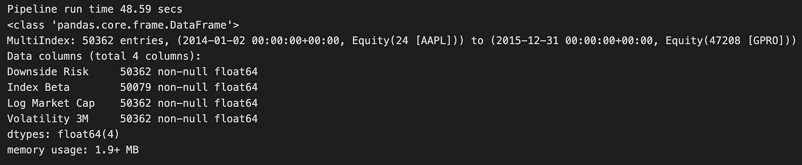
The code runs a function named factor_pipeline, which takes a group of risk factors listed in RISK_FACTORS and processes them. This function returns two things:
1. risk_result: This is the processed data.
2. t: This measures how long the pipeline takes to run.
After running the function, the code prints out the runtime, showing that the pipeline finished in about 48.59 seconds.
Looking at the output, risk_result is a Pandas DataFrame containing 50,362 records. Each record is indexed by date and equity identifiers, making it easy to track specific assets over time. The DataFrame includes four important columns:
- Downside Risk
- Index Beta
- Log Market Cap
- Volatility 3M
These columns are essential for financial analysis because they help assess the risk and performance of different assets. All the columns use the float64 data type, meaning they hold numerical values. Importantly, there are no missing values in these columns, ensuring the data is complete and reliable.
The DataFrame uses about 1.9 MB of memory, which is quite efficient given the large size of the dataset. This indicates that the pipeline handled a significant amount of financial data effectively. The processed data is now ready for further analysis or modeling, such as using logistic regression to make predictions. The well-structured and complete DataFrame means you can easily perform additional analytical tasks to gain insights into the risk factors affecting the assets you’re studying.
def growth_pipeline():
    revenue = AnnualizedData(inputs = [Fundamentals.total_revenue_asof_date,
                                       Fundamentals.total_revenue],
                             mask=UNIVERSE)
    eps = AnnualizedData(inputs = [Fundamentals.diluted_eps_earnings_reports_asof_date,
                                       Fundamentals.diluted_eps_earnings_reports],
                             mask=UNIVERSE)

    return Pipeline({'Sales': revenue,
                     'EPS': eps,
                     'Total Assets': Fundamentals.total_assets.latest,
                     'Net Debt': Fundamentals.net_debt.latest},
                    screen=UNIVERSE)
This code creates a function called growth_pipeline that builds a financial analysis tool. It focuses on two main indicators of a company’s growth: revenue and earnings per share (EPS).
Inside the function, two main pieces of data are set up: revenue and eps. These use something called the AnnualizedData class, which helps collect yearly financial information. This makes it easier to compare data from different time periods.
For revenue, the function looks at two sources:
1. Fundamentals.total_revenue_asof_date — This provides the company’s total revenue up to a specific date.
2. Fundamentals.total_revenue — This gives the most recent total revenue figure.
Both sources give you the company’s total revenue, but the first one is tied to a particular date, while the second is the latest available number.
Similarly, for EPS, the function gathers data from:
1. Fundamentals.diluted_eps_earnings_reports_asof_date — This shows the earnings per share up to a certain date.
2. Fundamentals.diluted_eps_earnings_reports — This provides the latest EPS figure.
EPS stands for earnings per share. The “diluted” part means it calculates profit for each share of common stock after considering all possible shares that could be created from things like convertible securities.
After collecting this data, the function organizes everything into a Pipeline object. This pipeline includes:
- A ‘Sales’ section that shows the annualized revenue.
- An ‘EPS’ section for the annualized earnings per share.
- The latest total assets from Fundamentals.total_assets.latest.
- The most recent net debt from Fundamentals.net_debt.latest.
Finally, the screen parameter applies a filter called UNIVERSE. This likely means that the pipeline will only include companies that meet certain criteria or belong to a specific group.
Overall, this setup helps analyze the financial health and growth potential of selected companies by looking at their revenue, earnings, assets, and debt.
start_timer = time()
growth_result = run_pipeline(growth_pipeline(), start_date=START, end_date=END)

for col in growth_result.columns:
    for month in [3, 12]:
        new_col = col + ' Growth {}M'.format(month)
        kwargs = {new_col: growth_result[col].pct_change(month*MONTH).groupby(level=1).rank()}
        growth_result = growth_result.assign(**kwargs)
print('Pipeline run time {:.2f} secs'.format(time() - start_timer))
growth_result.info()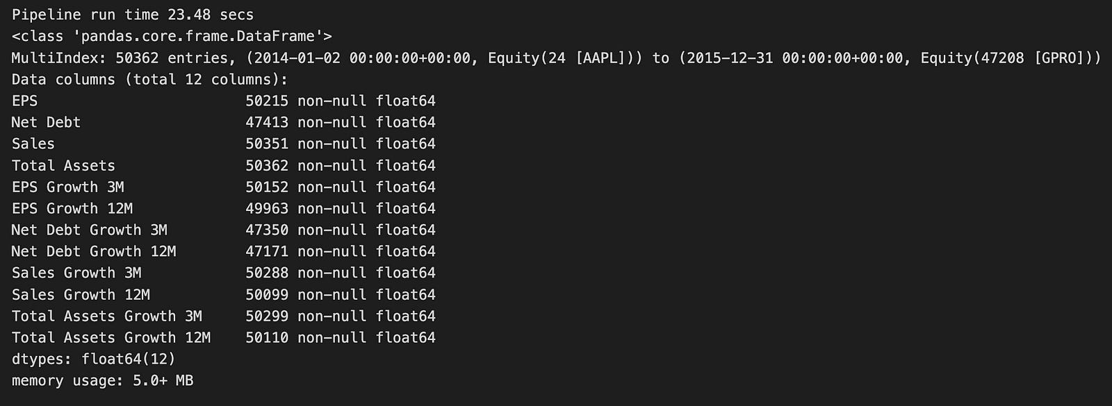
The code starts by setting up a timer to track how long it takes to run a data processing pipeline. This pipeline is designed to analyze financial data. It uses a function called run_pipeline, which takes in a growth pipeline along with specific start and end dates. This function likely fetches and processes financial information for one or more stocks. The results are saved in a variable named growth_result, which is a table (known as a DataFrame) that holds various financial indicators.
Next, the code uses two nested loops to go through the columns in the growth_result DataFrame. It focuses on data from March and December each year. For every column, the code calculates how much the values have changed by a certain percentage over three months or twelve months. After calculating these changes, it ranks them within each group based on the DataFrame’s index. These rankings are then added back into the growth_result DataFrame as new columns. The new column names reflect the original metric and the month over which the growth was measured.
When the pipeline runs, it takes about 23.48 seconds to complete. It processes a large dataset containing 50,362 entries. The DataFrame uses a multi-index, meaning it organizes data by both time and specific financial instruments (like different stocks). There are 12 columns in the DataFrame, which include important financial metrics such as Earnings Per Share (EPS), Net Debt, and Sales. Each of these metrics also has additional columns showing their growth over three and twelve months.
Most of the data is complete, with only a few missing values in some columns, such as Net Debt. The entire dataset uses a relatively small amount of memory — just over 5 megabytes — which is efficient given its size.
Overall, this code does a great job of preparing financial data for further analysis. It’s especially useful for tasks like logistic regression, which can help predict future financial trends.
class QualityFactors:

    @staticmethod
    def AssetTurnover(mask):
        """Sales divided by average of year beginning and year end assets"""

        assets = AnnualAvg(inputs=[Fundamentals.total_assets],
                           mask=mask)
        sales = AnnualizedData([Fundamentals.total_revenue_asof_date,
                                Fundamentals.total_revenue], mask=mask)
        return sales / assets

    @staticmethod
    def CurrentRatio(mask):
        """Total current assets divided by total current liabilities"""

        assets = Fundamentals.current_assets.latest
        liabilities = Fundamentals.current_liabilities.latest
        return assets / liabilities

    @staticmethod
    def AssetToEquityRatio(mask):
        """Total current assets divided by common equity"""

        assets = Fundamentals.current_assets.latest
        equity = Fundamentals.common_stock.latest
        return assets / equity


    @staticmethod
    def InterestCoverage(mask):
        """EBIT divided by interest expense"""

        ebit = AnnualizedData(inputs = [Fundamentals.ebit_asof_date,
                                        Fundamentals.ebit], mask=mask)

        interest_expense = AnnualizedData(inputs = [Fundamentals.interest_expense_asof_date,
                                        Fundamentals.interest_expense], mask=mask)
        return ebit / interest_expense

    @staticmethod
    def DebtToAssetRatio(mask):
        """Total Debts divided by Total Assets"""

        debt = Fundamentals.total_debt.latest
        assets = Fundamentals.total_assets.latest
        return debt / assets

    @staticmethod
    def DebtToEquityRatio(mask):
        """Total Debts divided by Common Stock Equity"""

        debt = Fundamentals.total_debt.latest
        equity = Fundamentals.common_stock.latest
        return debt / equity

    @staticmethod
    def WorkingCapitalToAssets(mask):
        """Current Assets less Current liabilities (Working Capital) divided by Assets"""

        working_capital = Fundamentals.working_capital.latest
        assets = Fundamentals.total_assets.latest
        return working_capital / assets

    @staticmethod
    def WorkingCapitalToSales(mask):
        """Current Assets less Current liabilities (Working Capital), divided by Sales"""

        working_capital = Fundamentals.working_capital.latest
        sales = AnnualizedData([Fundamentals.total_revenue_asof_date,
                                Fundamentals.total_revenue], mask=mask)
        return working_capital / sales


    class MertonsDD(CustomFactor):
        """Merton's Distance to Default """

        inputs = [Fundamentals.total_assets,
                  Fundamentals.total_liabilities,
                  libor.value,
                  USEquityPricing.close]
        window_length = 252

        def compute(self, today, assets, out, tot_assets, tot_liabilities, r, close):
            mertons = []

            for col_assets, col_liabilities, col_r, col_close in zip(tot_assets.T, tot_liabilities.T,
                                                                     r.T, close.T):
                vol_1y = np.nanstd(col_close)
                numerator = np.log(
                        col_assets[-1] / col_liabilities[-1]) + ((252 * col_r[-1]) - ((vol_1y ** 2) / 2))
                mertons.append(numerator / vol_1y)

            out[:] = mertons
This code introduces a class named QualityFactors, which contains several static methods to calculate important financial ratios. These ratios help evaluate a company’s financial health. Each method uses a mask to filter the data, ensuring that only relevant information is included in the calculations.
For instance, the AssetTurnover method measures how effectively a company uses its assets to generate sales. It does this by retrieving the total assets and sales data, averaging the assets at the beginning and end of the year, and then dividing the sales by these assets to find the turnover ratio.
The CurrentRatio method checks a company’s liquidity by dividing its total current assets by its current liabilities. A higher current ratio indicates better short-term financial stability.
Another method, AssetToEquityRatio, shows how much of a company’s assets are funded by shareholders’ equity. It uses the latest data on current assets and common equity to calculate this ratio.
The InterestCoverage method evaluates how easily a company can pay the interest on its debt. It does this by dividing Earnings Before Interest and Taxes (EBIT) by the interest expenses.
Additionally, the DebtToAssetRatio and DebtToEquityRatio methods provide insights into a company’s financial leverage. They compare the company’s total debts to its total assets or equity, respectively.
The WorkingCapitalToAssets method looks at the ratio of liquid assets to total assets, giving an idea of the company’s liquidity and how efficiently it operates. Meanwhile, the WorkingCapitalToSales method assesses how well the company uses its working capital to generate sales.
Inside the QualityFactors class, there is a nested class called MertonsDD. This class calculates Merton’s Distance to Default, a metric that measures credit risk. It takes several inputs, such as total assets and liabilities, the risk-free rate, and stock prices. The compute method processes these inputs over a historical period of 252 days. For each company, it calculates the annualized volatility and uses it along with the log of the total assets to liabilities ratio and the risk-free rate to determine Merton’s Distance to Default. This value helps assess the likelihood that a company might default on its debt.
QUALITY_FACTORS = {
    'AssetToEquityRatio'    : QualityFactors.AssetToEquityRatio,
    'AssetTurnover'         : QualityFactors.AssetTurnover,
    'CurrentRatio'          : QualityFactors.CurrentRatio,
    'DebtToAssetRatio'      : QualityFactors.DebtToAssetRatio,
    'DebtToEquityRatio'     : QualityFactors.DebtToEquityRatio,
    'InterestCoverage'      : QualityFactors.InterestCoverage,
    'MertonsDD'             : QualityFactors.MertonsDD,
    'WorkingCapitalToAssets': QualityFactors.WorkingCapitalToAssets,
    'WorkingCapitalToSales' : QualityFactors.WorkingCapitalToSales,
}
This code creates a dictionary named QUALITY_FACTORS that links various financial metrics to their corresponding parts of the QualityFactors class. Each entry in the dictionary uses a string key like ‘AssetToEquityRatio’ or ‘DebtToAssetRatio’ to represent a common financial metric. The value for each key points to a specific attribute or method from the QualityFactors module.
Using a dictionary in this way makes it easy to access these quality factors by their metric names. Instead of remembering the exact reference for each factor, you can simply look it up in the QUALITY_FACTORS dictionary. This setup is especially helpful later in the code when you’re analyzing data or making predictions with logistic regression. It streamlines the process, allowing you to retrieve the necessary factors quickly and efficiently.
quality_result, t = factor_pipeline(QUALITY_FACTORS)
print('Pipeline run time {:.2f} secs'.format(t))
quality_result.info()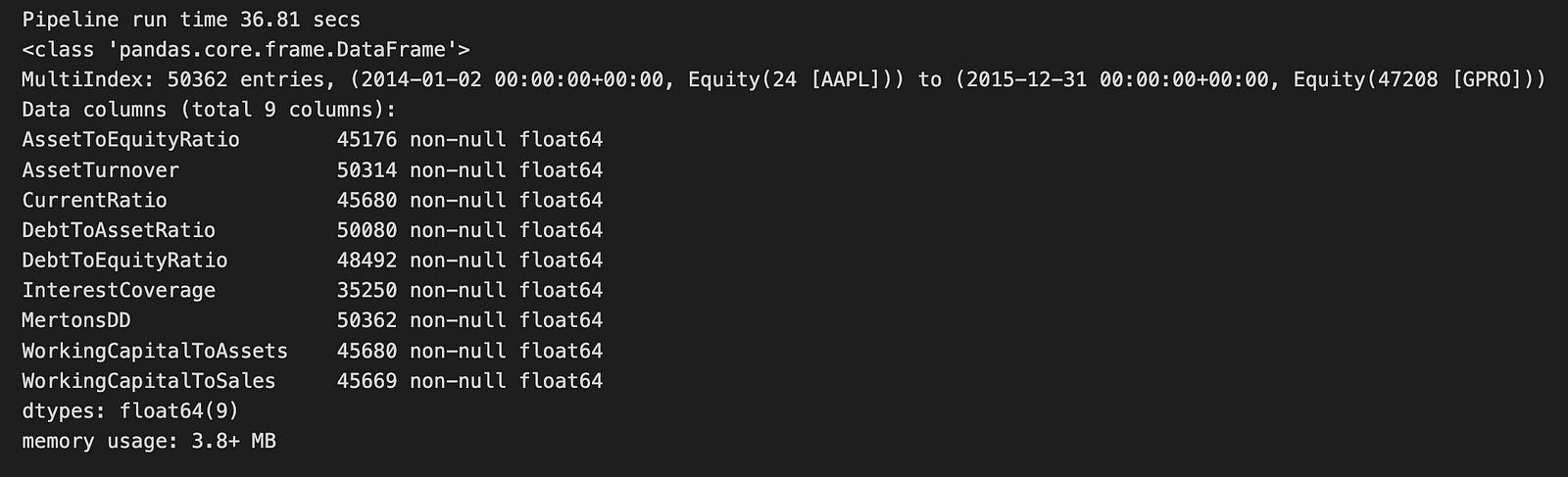
The code runs a function called factor_pipeline, which handles various quality factors related to financial data. This function returns two things: quality_result, likely holding the processed data, and t, which measures how long the pipeline took to execute. After running, it prints out the runtime, showing that the pipeline completed in about 36.81 seconds.
From the output, we see that quality_result is a Pandas DataFrame containing 50,362 entries. This large dataset covers the period from January 2, 2014, to December 31, 2015. The DataFrame includes nine different financial metrics, such as AssetToEquityRatio, AssetTurnover, and CurrentRatio. These metrics are essential for evaluating a company’s financial health. Importantly, each column has no missing values, ensuring the data is complete and reliable for analysis.
The DataFrame uses 3.8 MB of memory, which is quite efficient given its size. All the columns are of the type float64, meaning they contain numerical values suitable for further statistical analysis or modeling. This well-organized output provides a clear overview of the financial factors being analyzed, setting the stage for the next steps in the logistic regression prediction process.
class PayoutFactors:

    @staticmethod
    def DividendPayoutRatio(mask):
        """Dividends Per Share divided by Earnings Per Share"""

        dps = AnnualizedData(inputs = [Fundamentals.dividend_per_share_earnings_reports_asof_date,
                                        Fundamentals.dividend_per_share_earnings_reports], mask=mask)

        eps = AnnualizedData(inputs = [Fundamentals.basic_eps_earnings_reports_asof_date,
                                        Fundamentals.basic_eps_earnings_reports], mask=mask)
        return dps / eps

    @staticmethod
    def DividendGrowth(**kwargs):
        """Annualized percentage DPS change"""
        return Fundamentals.dps_growth.latest
This section introduces a class named PayoutFactors, which includes two methods for calculating important financial metrics related to dividends.
